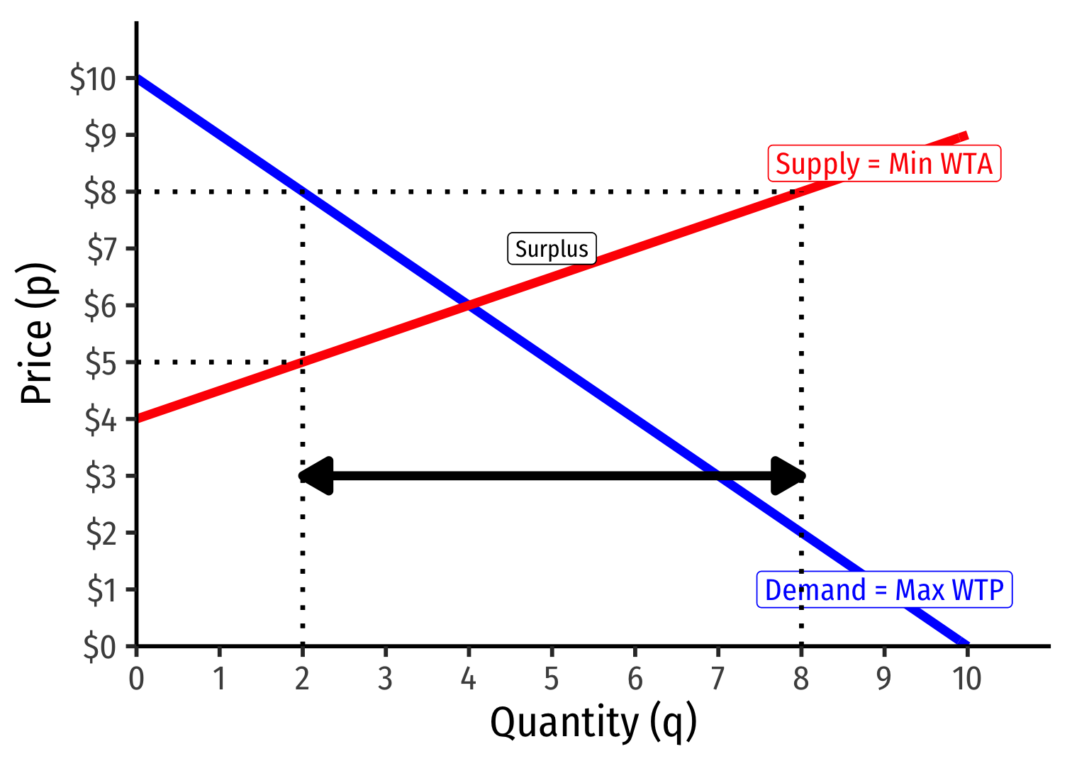
Excess Demand I
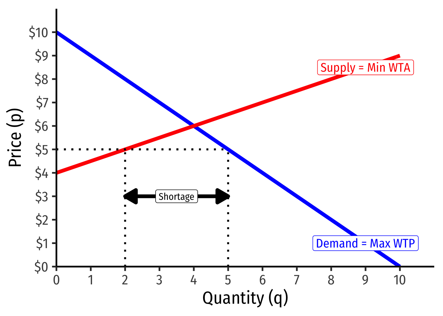
Example: Consider any price below $6, such as $5:
Qd=5Qs=2
Qd>Qs: excess demand
A shortage of 3 units
Excess Demand II
Example: Consider any price below $6, such as $5:
Qd=5Qs=2
Qd>Qs: excess demand
A shortage of 3 units
Sellers will not supply more than 2 units
For 2 units, some buyers are willing to pay more than $5
Excess Demand III
Example: Consider any price below $6, such as $5:
Qd=5Qs=2
Qd>Qs: excess demand
A shortage of 3 units
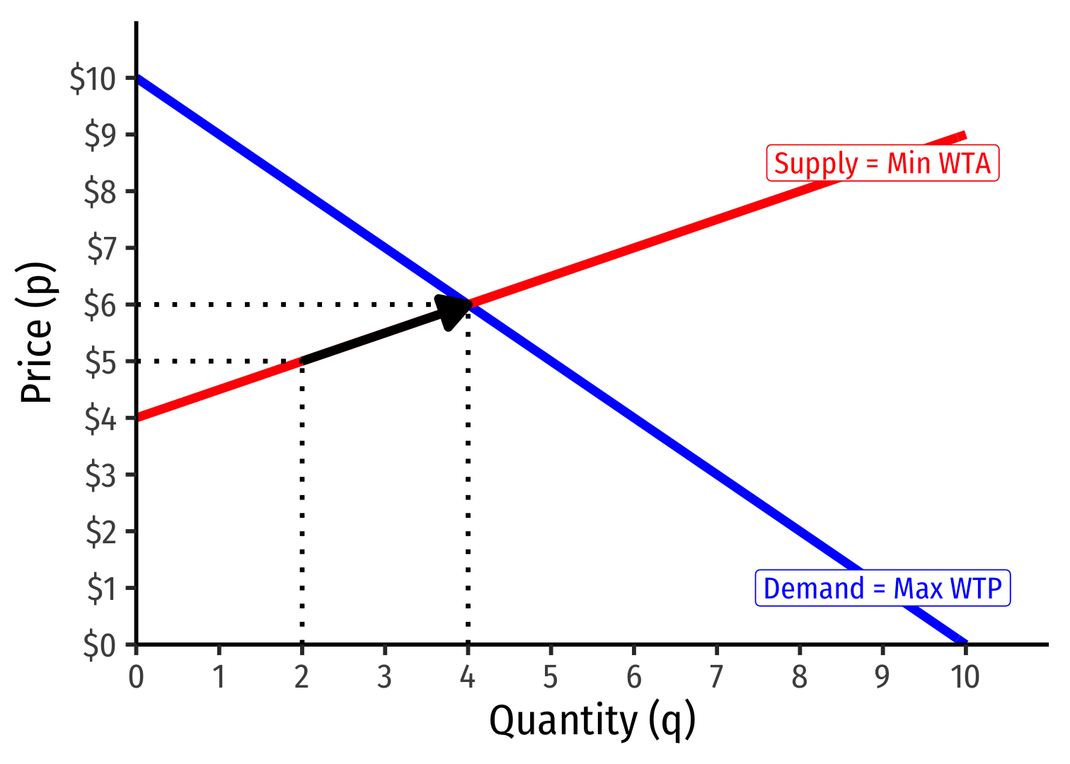
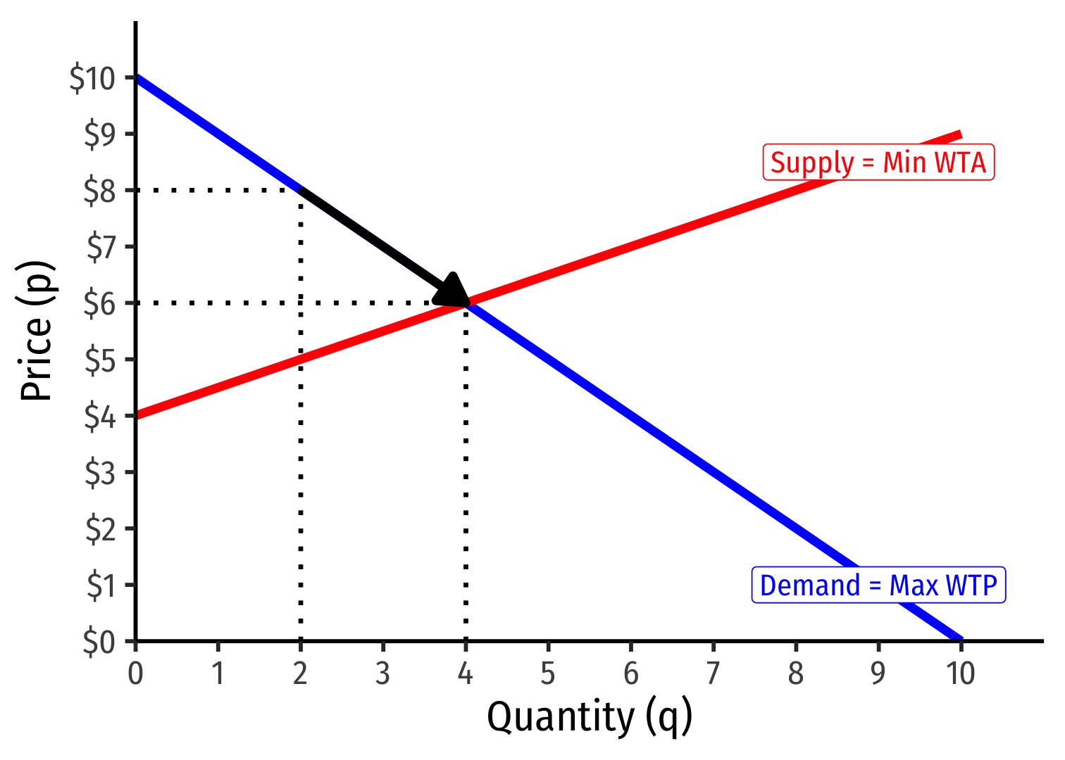
Buyers will raise their bids against one another, raising the price
At higher prices, sellers are willing to supply more!
Continues until equilibrium, no pressure for change, qs=qd
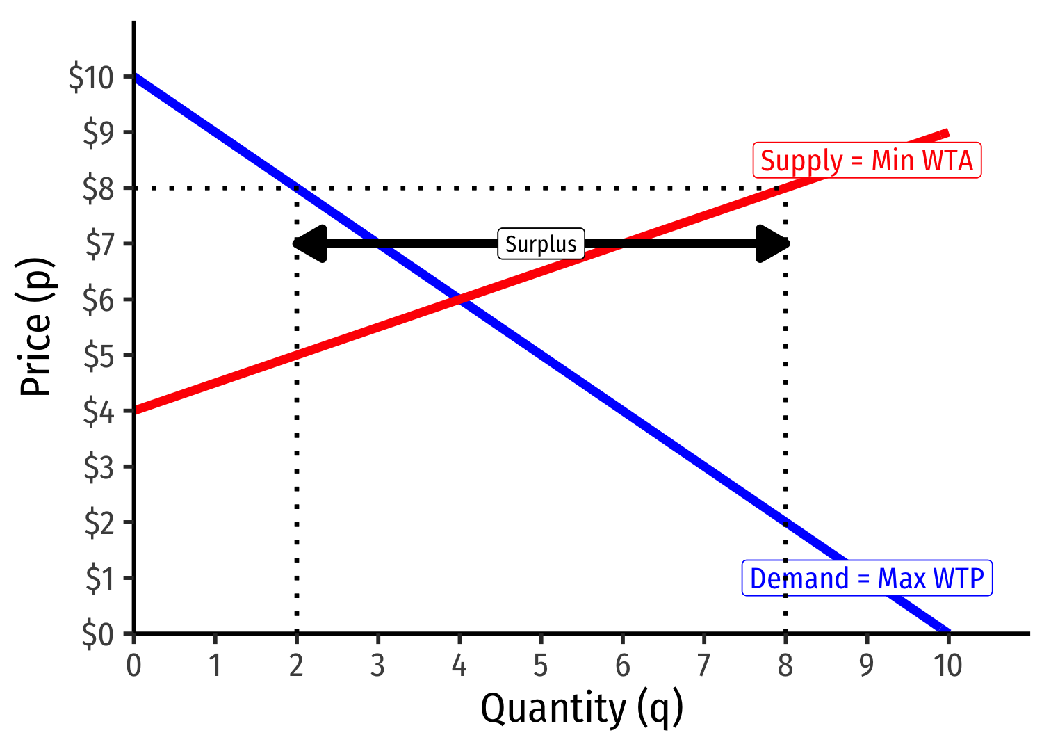
Excess Supply I
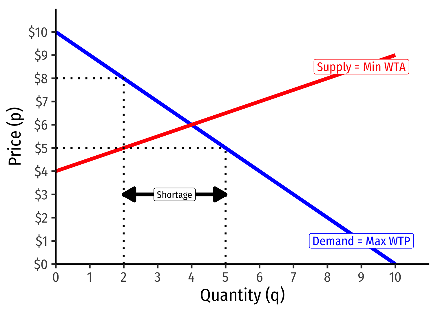
Example: Consider any price above $6, such as $8:
Qd=2;Qs=8
Qd<Qs: excess supply
A surplus of 6 units
Excess Supply II
Example: Consider any price above $6, such as $8:
Qd=2;Qs=8
Qd<Qs: excess supply
A surplus of 6 units
Buyers will not buy more than 2 units
For 2 units, some sellers are willing to accept less than $8
Excess Supply III
Example: Consider any price above $6, such as $8:
Qd=2;Qs=8
Qd<Qs: excess supply
A surplus of 6 units
Sellers will lower their asking prices against one another, lowering the price
At lower prices, buyers are willing to buy more!
Continues until equilibrium, no pressure for change, qs=qd
Why Markets Tend to Equilibrate

Ceterus Paribus I
Supply function and demand function relate quantity (supplied or demanded) to price only
- Describes how buyers/sellers respond to changes in market price
Certainly there are many other factors that influence how much a buyer or seller will purchase at a particular price!
- income, preferences, prices of other goods, expectations, etc.
A supply or demand function (or graph) requires "ceterus paribus" (all else equal)

Recall (for example), Demand I
- A consumer's quantity demanded (of good x), qDx is a function of their demand for good x, which depends on current market prices and their income
qDx=D(m,px,py)
- Income effects (ΔqDxΔm): how qDx changes with changes in income
- Cross-price effects (ΔqDxΔpy): how qDx changes with changes in prices of other goods (e.g. y)
- (Own) Price effects (ΔqDxΔpx): how qDx changes with changes in price (of x)

See Class 1.7 for a reminder.
Recall (for example), Demand II
A change in one of the "determinants of demand" (or "shifters") will shift the demand curve
- Change in income m
- Change in price of other goods py (substitutes or complements)
- Change in preferences or expectations about good x (show up in utility function)
- Change in number of buyers in market
Shows up in (inverse) demand function by a change in the intercept (choke price)!
See my Visualizing Demand Shifters
See Class 1.9 for a reminder.
Ceterus Paribus II
Consider our demand function: qD=10−p
If the market price (p) changes (perhaps because supply changes), that results in a change in quantity demanded (qD)
- We move along the existing demand curve
Ceterus paribus has not been violated
Ceterus Paribus III
Consider our demand function: qD=10−p
If the something other than price changes (income, preferences, price of a complement, etc), that results in a change in demand
- We need to draw a new demand curve (or demand function)
qD=12−p
- Ceterus paribus has been violated
Ceterus Paribus IV
- There is a big difference between a change in "quantity demanded" and a change in "demand"!

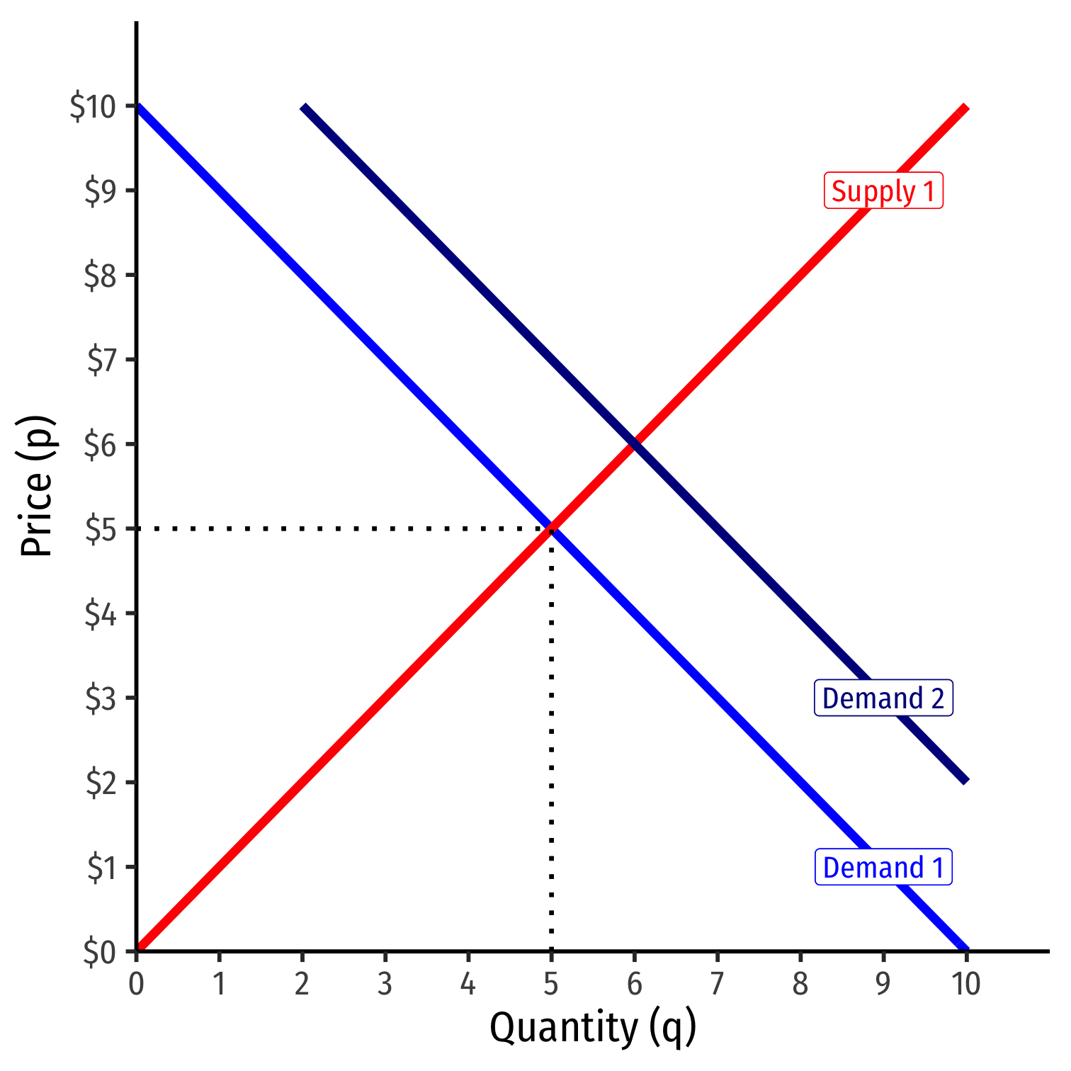
Increase in Demand

Increase in Demand
More individuals want to buy more of the good at every price
Entire demand curve shifts to the right
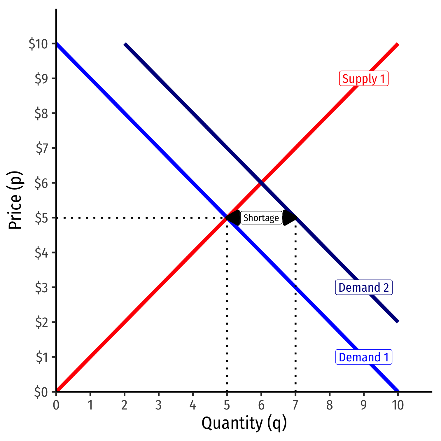
Increase in Demand
More individuals want to buy more of the good at every price
Entire demand curve shifts to the right
At the original market price, a shortage! (qD>qS)
Increase in Demand
More individuals want to buy more of the good at every price
Entire demand curve shifts to the right
At the original market price, a shortage! (qD>qS)
Some buyers willing to pay more at this quantity

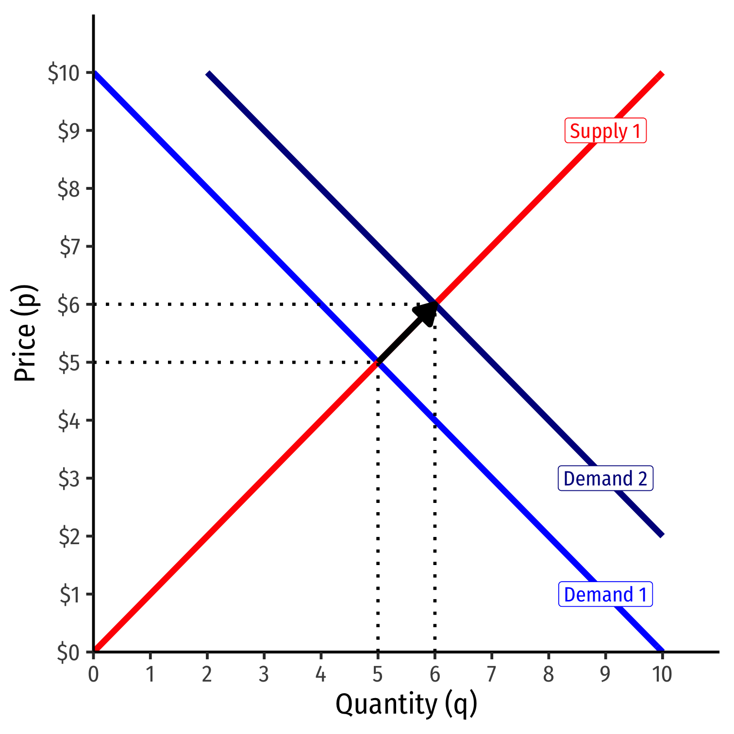
Increase in Demand
More individuals want to buy more of the good at every price
Entire demand curve shifts to the right
At the original market price, a shortage! (qD>qS)
Some buyers willing to pay more at this quantity
Buyers raise bids, inducing sellers to sell more
Reach new equilibrium with:
- higher market-clearing price
- larger market-clearing quantity exchanged
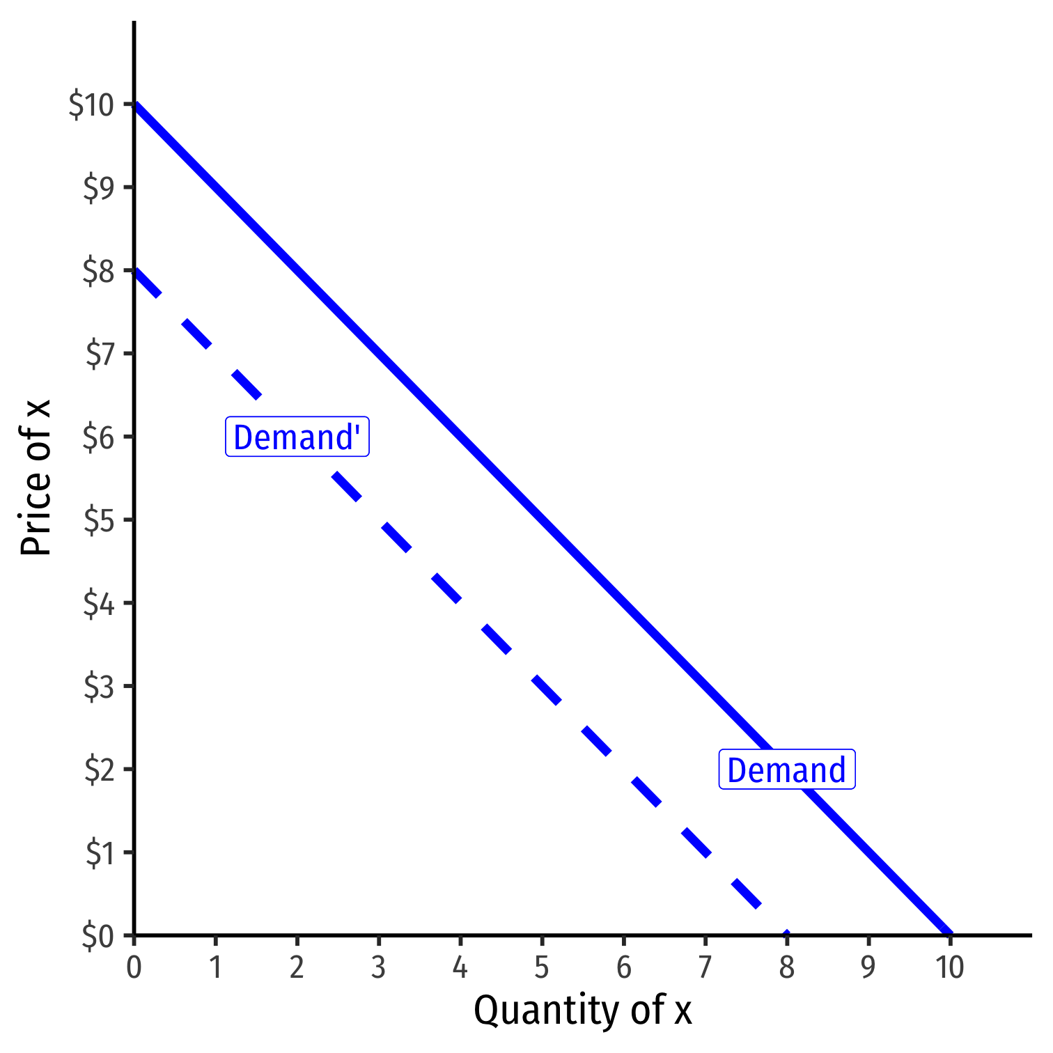
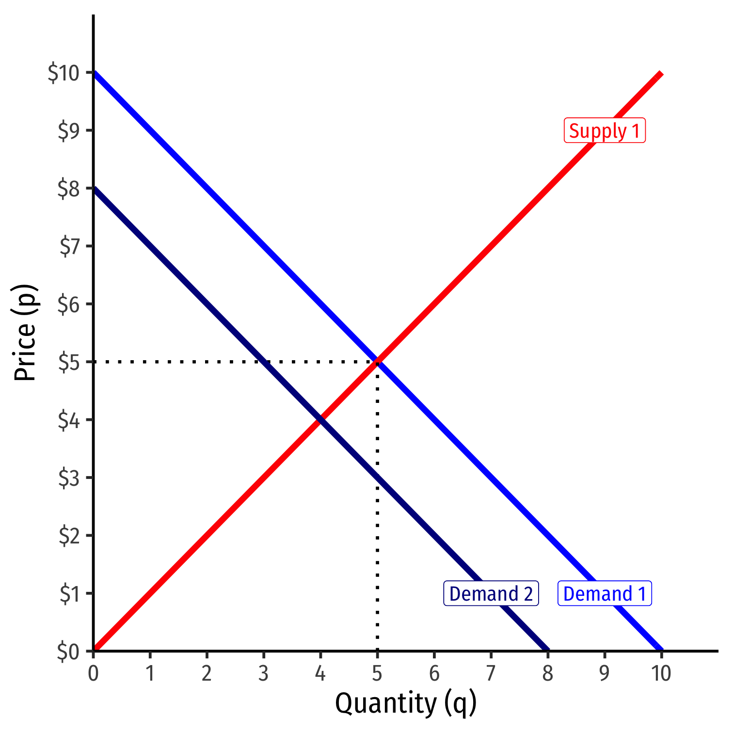
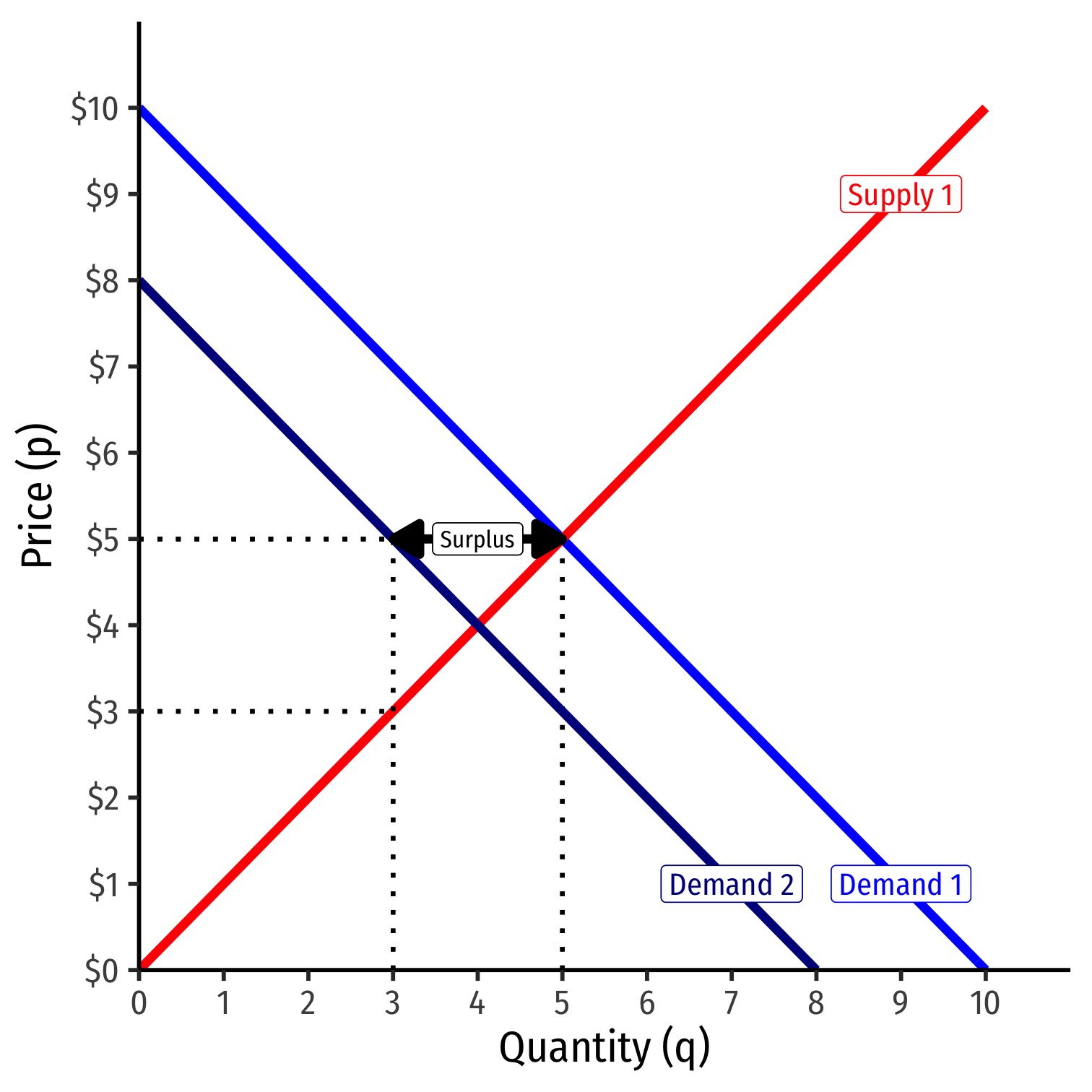
Decrease in Demand

Decrease in Demand
Fewer individuals want to buy less of the good at every price
Entire demand curve shifts to the left
Increase in Demand
Fewer individuals want to buy less of the good at every price
Entire demand curve shifts to the left
At the original market price, a surplus! (qD<qS)

Decrease in Demand
Fewer individuals want to buy less of the good at every price
Entire demand curve shifts to the left
At the original market price, a surplus! (qD<qS)
Some sellers willing to accept less at this quantity
Increase in Demand
Fewer individuals want to buy less of the good at every price
Entire demand curve shifts to the left
At the original market price, a surplus! (qD<qS)
Some sellers willing to accept less at this quantity
Sellers lower asks, inducing buyers to buy more
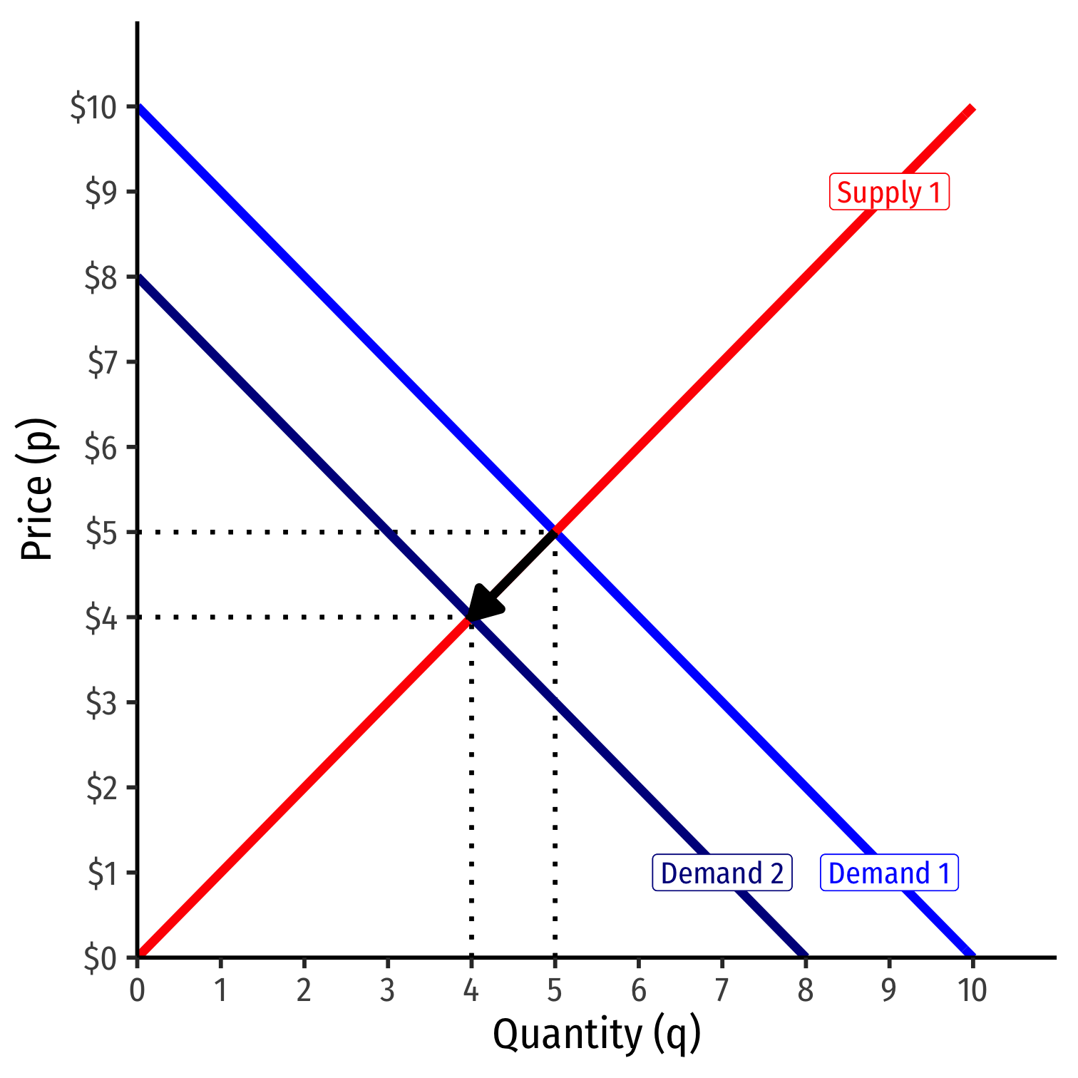
Reach new equilibrium with:
- lower market-clearing price
- smaller market-clearing quantity exchanged
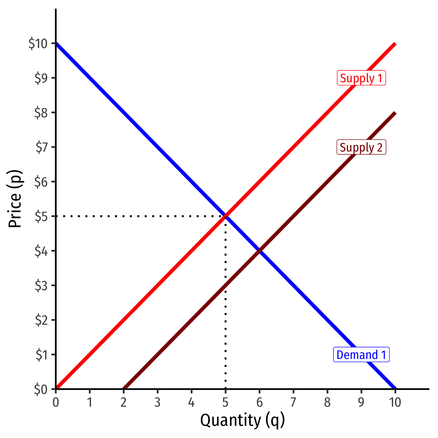
Increase in Supply

Increase in Supply
More individuals want to sell more of the good at every price
Entire supply curve shifts to the right
Increase in Supply
More individuals want to sell more of the good at every price
Entire supply curve shifts to the right
At the original market price, a surplus! (qD<qS)
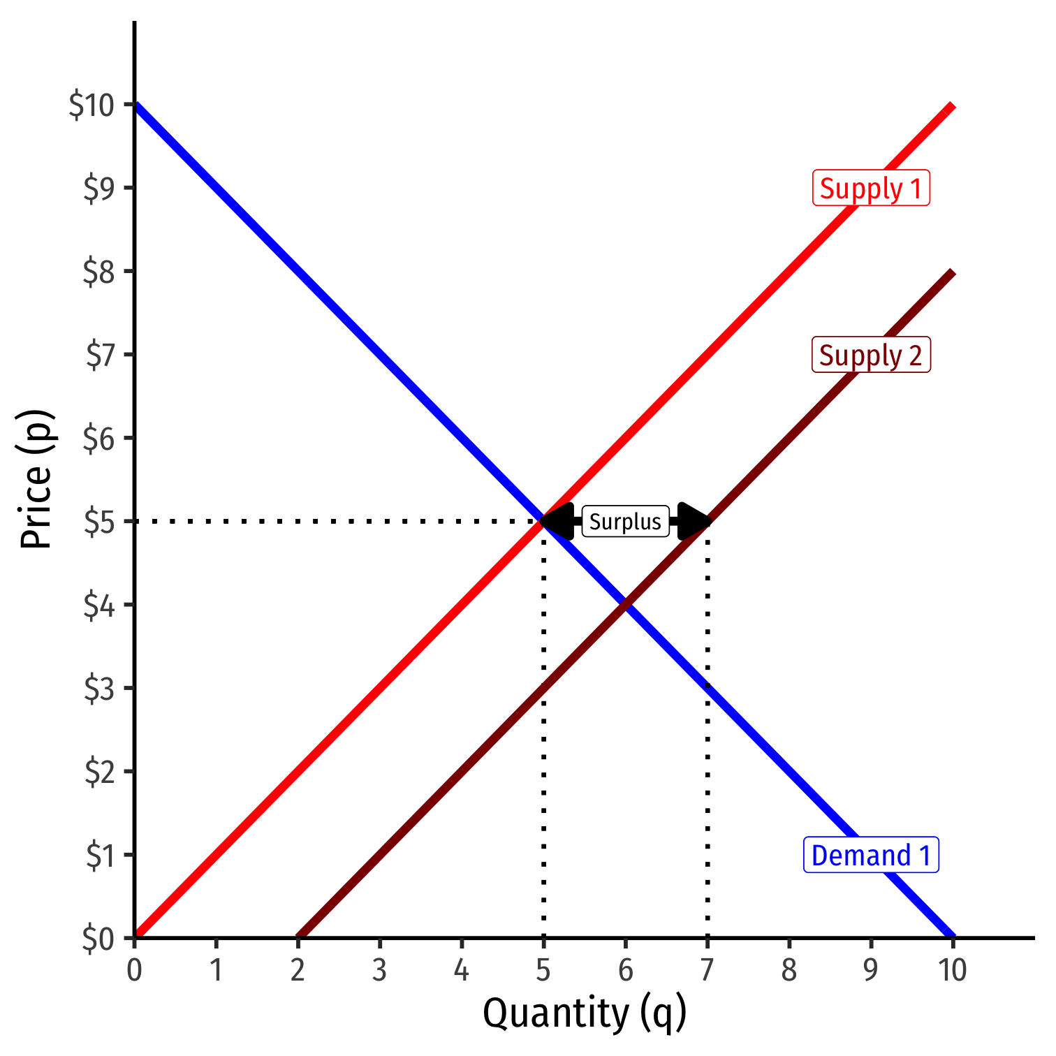
Increase in Supply
More individuals want to sell more of the good at every price
Entire supply curve shifts to the right
At the original market price, a surplus! (qD<qS)
Some sellers willing to accept less at this quantity

Increase in Supply
More individuals want to sell more of the good at every price
Entire supply curve shifts to the right
At the original market price, a surplus! (qD<qS)
Some sellers willing to accept less at this quantity
Sellers lower asks, inducing buyers to buy more
Reach new equilibrium with:
- lower market-clearing price
- larger market-clearing quantity exchanged
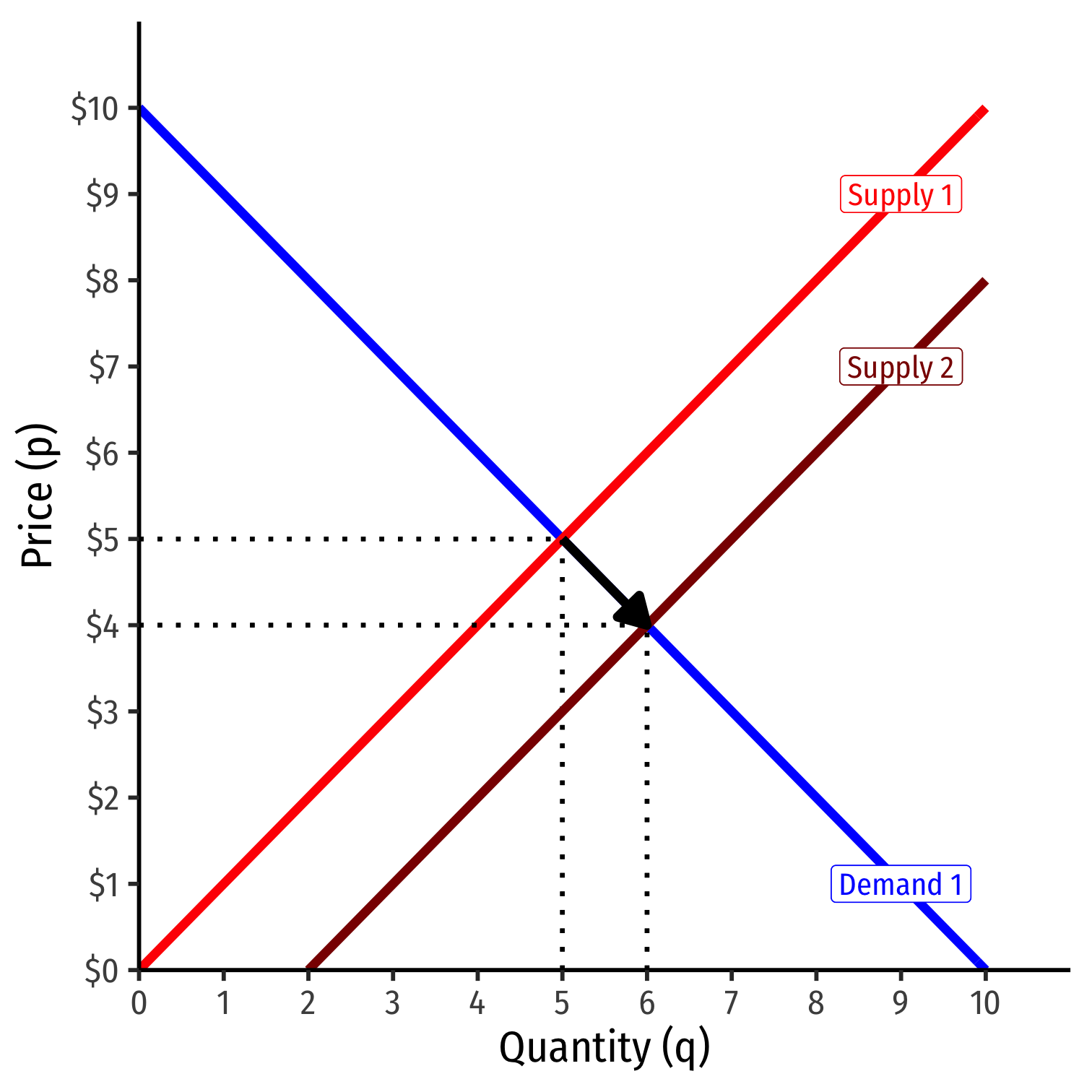
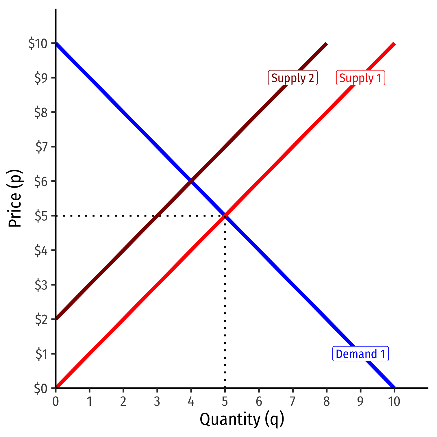
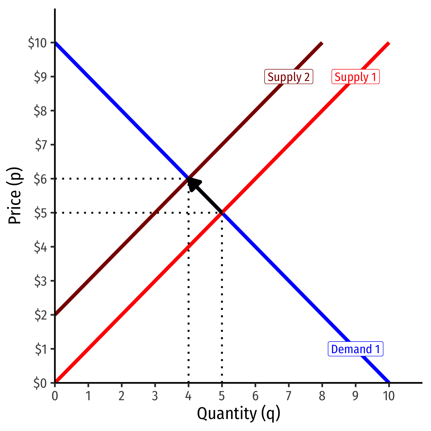
Decrease in Supply
Decrease in Supply
Fewer individuals want to sell less of the good at every price
Entire supply curve shifts to the left
Decrease in Supply
Fewer individuals want to sell less of the good at every price
Entire supply curve shifts to the left
At the original market price, a shortage! (qD>qS)
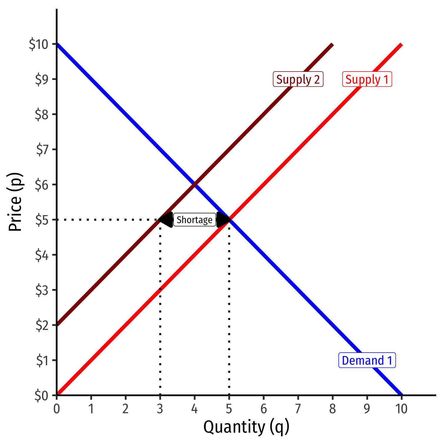
Decrease in Supply
Fewer individuals want to sell less of the good at every price
Entire supply curve shifts to the left
At the original market price, a shortage! (qD>qS)
Some buyers willing to pay more at this quantity

Decrease in Supply
Fewer individuals want to sell less of the good at every price
Entire supply curve shifts to the left
At the original market price, a shortage! (qD>qS)
Some buyers willing to pay more at this quantity
Buyers raise bids, inducing sellers to sell more
Reach new equilibrium with:
- higher market-clearing price
- smaller market-clearing quantity exchanged
Price Competition in Markets I
Markets allocate resources based on individuals' reservation prices:
- maximum willingness to pay (as a buyer)
- minimum willingness to accept (as a seller)
Goods flow to those who value them the highest and away from those who value them the lowest

Price Competition in Markets II
It might look like it, but competition in markets is NOT between buyers vs. sellers!
In markets: buyers compete with other buyers and sellers compete with other sellers

Price Competition in Markets III
Buyers want to pay the lowest price to buy a good
But they face competition from other buyers over the same scarce goods
Buyers attempt to raise their bids above others' reservation prices to obtain the goods
Price Competition in Markets IV
Sellers want to get the highest price for a good they sell
But they face competition from other sellers over the same potential customers
Sellers attempt to lower their asking prices below others' reservation prices to sell their goods
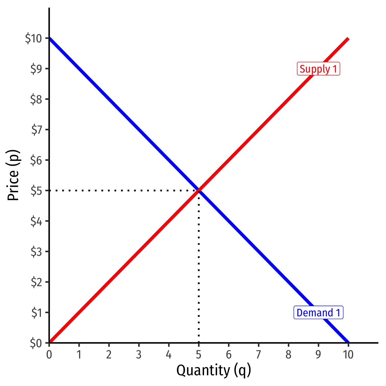
Market-Clearing Prices
- Supply and demand set the market-clearing price for all units exchanged (bought and sold)

Consumer Surplus I
Demand function measures how much you would hypothetically be willing to pay for various quantities
- "reservation price"
You often actually pay (the market-clearing price, p∗) a lot less than your reservation price
The difference is consumer surplus
CS=WTP−p∗

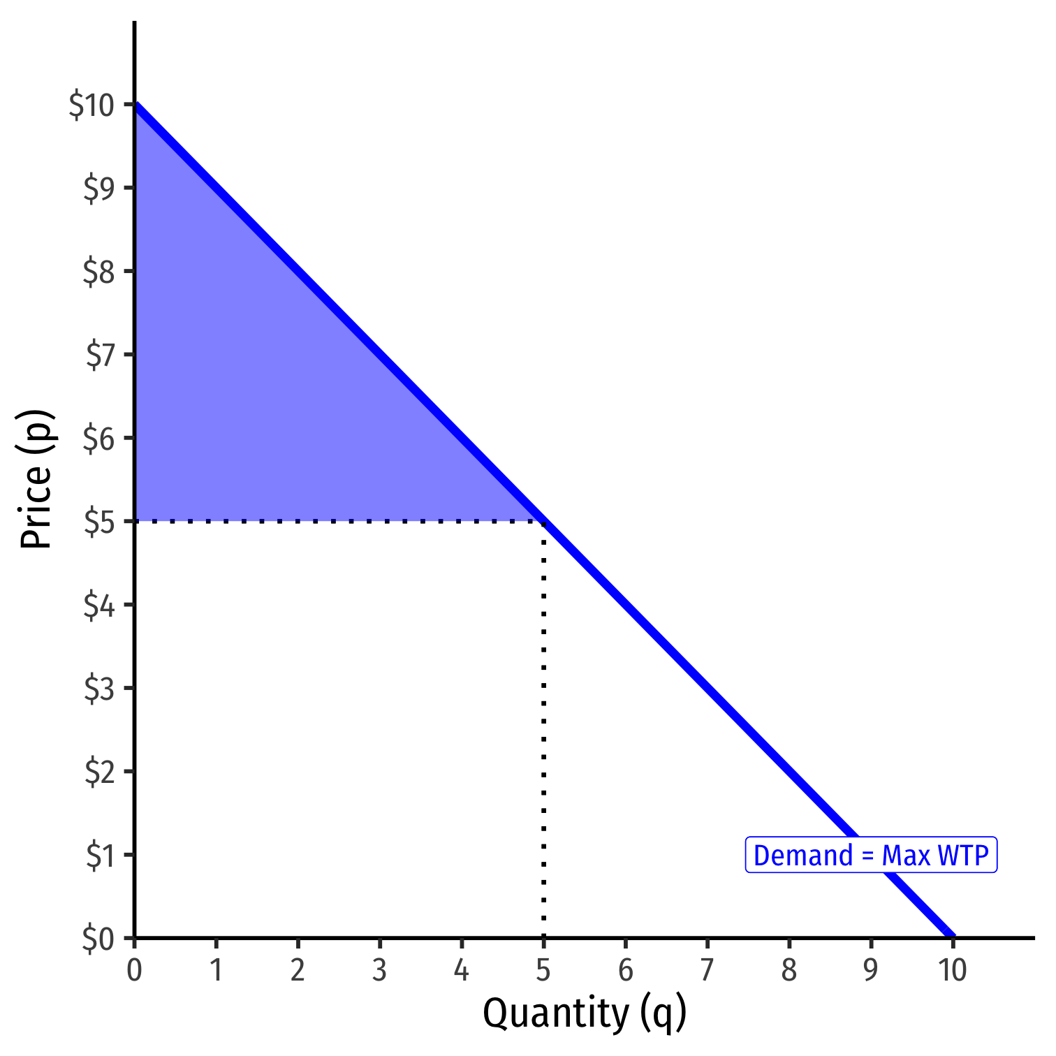
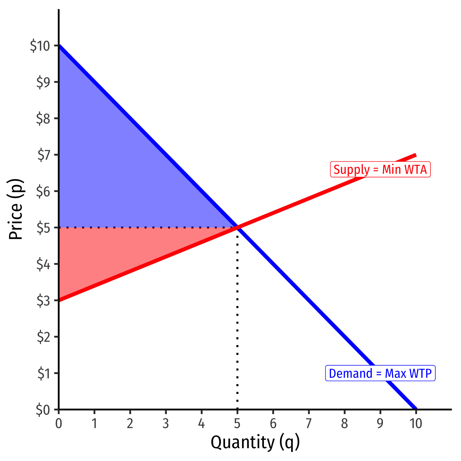
Consumer Surplus II
CS=12bhCS=12(5−0)($10−$5)CS=$12.50

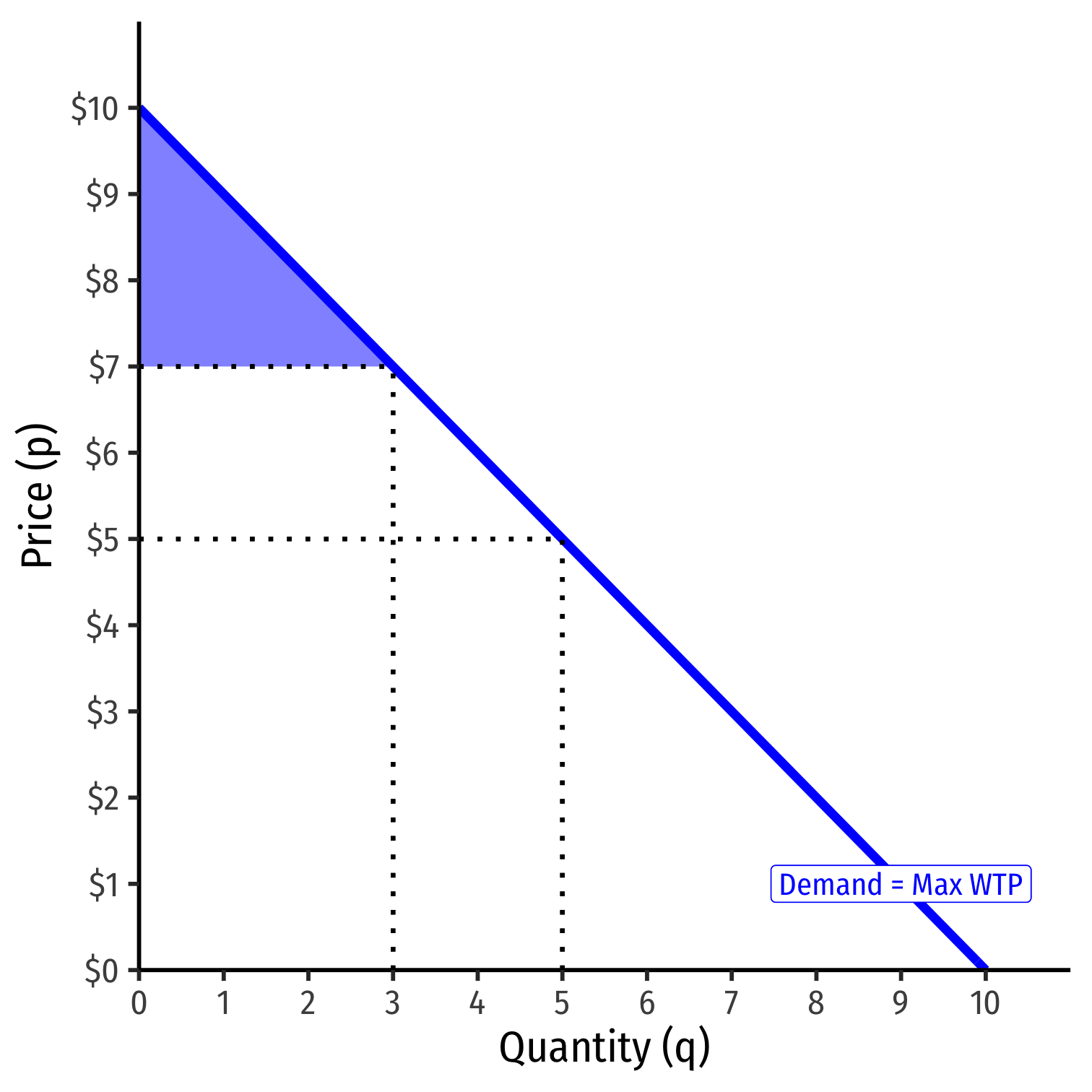
Consumer Surplus III
- An increase in market price reduces consumer surplus
CS′=12bhCS′=12(3−0)($10−$7)CS′=$4.50
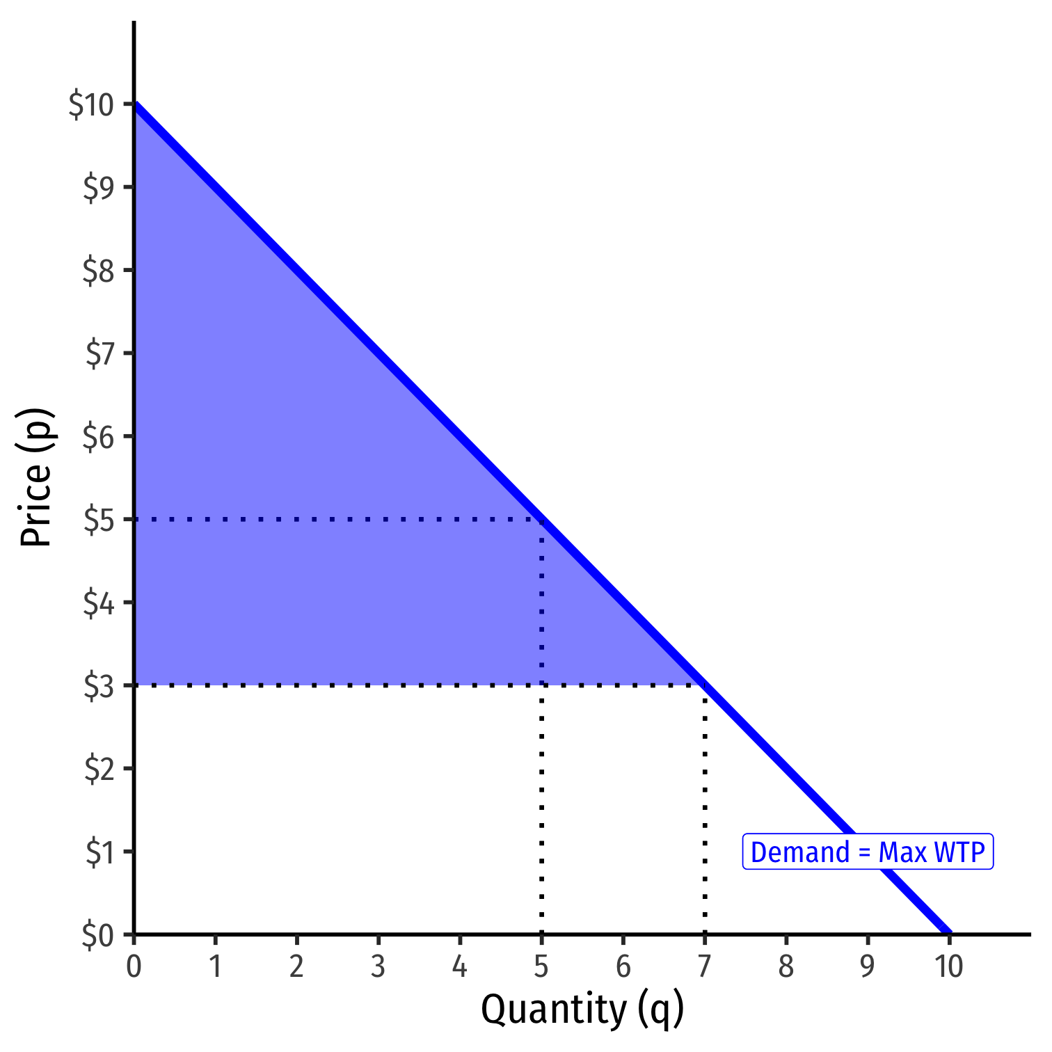
Consumer Surplus IV
- An decrease in market price increases consumer surplus
CS′=12bhCS′=12(7−0)($10−$3)CS′=$24.50
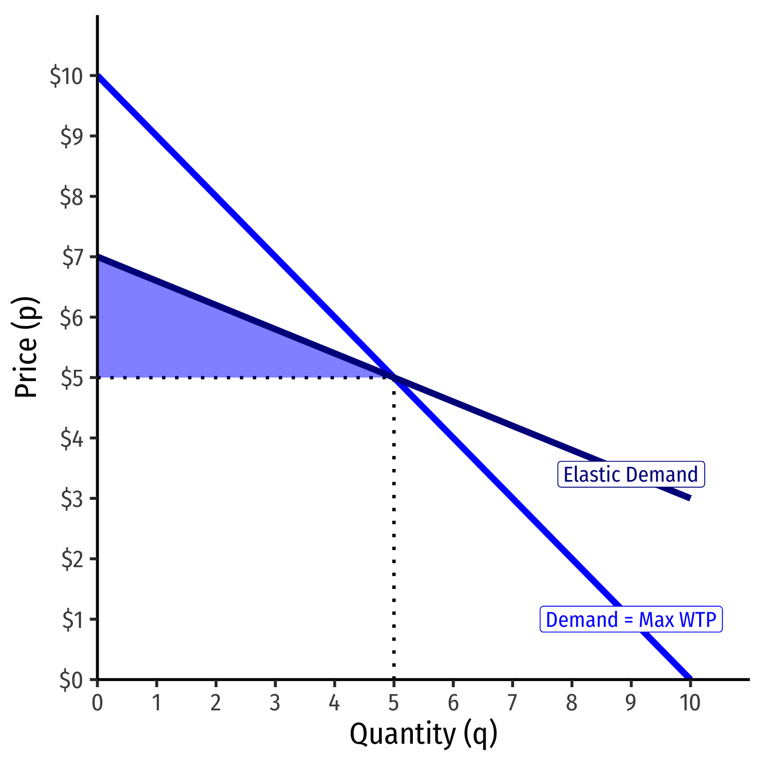
Consumer Surplus V
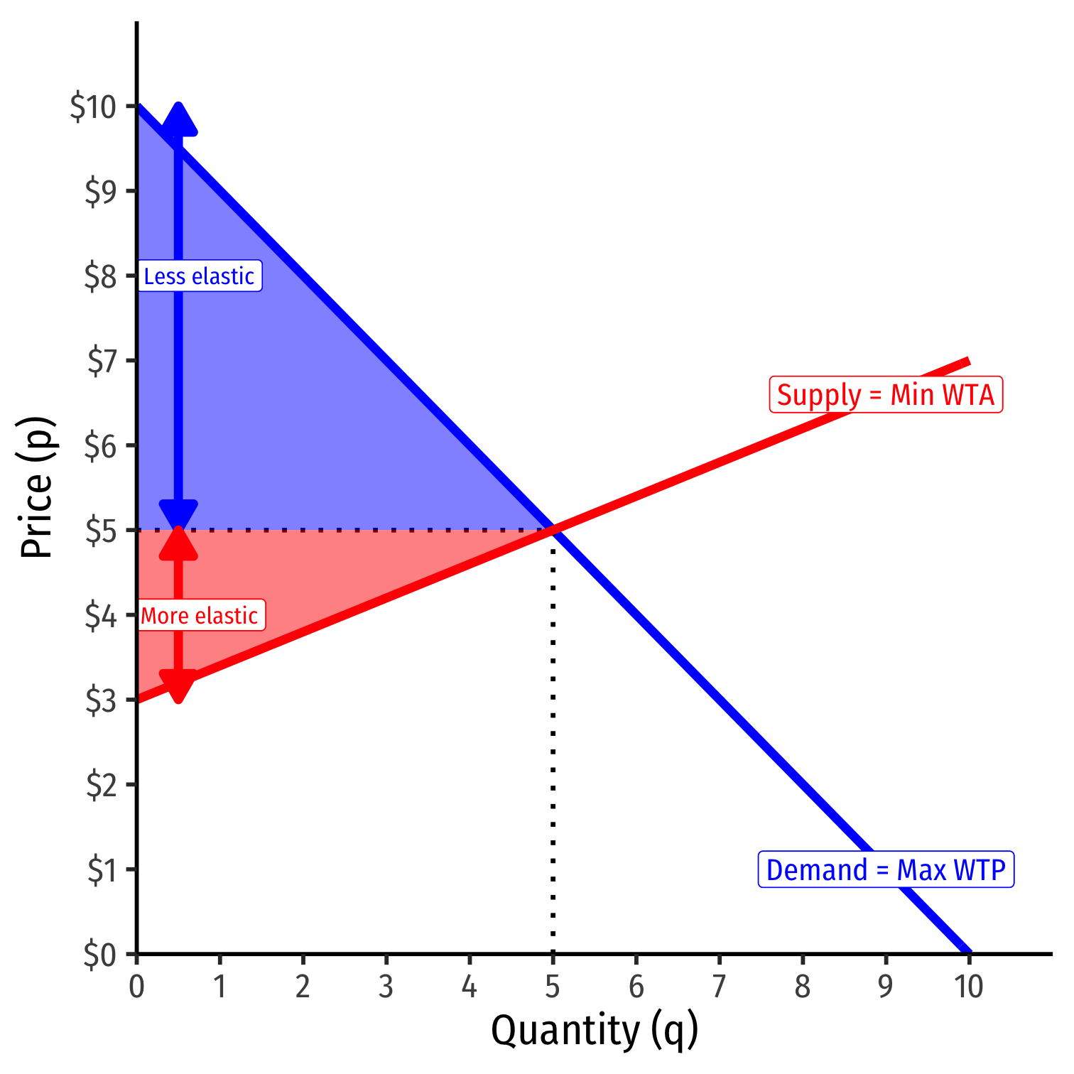
- A relatively inelastic demand curve generates more consumer surplus
CS=12bhCS=12(5−0)($10−$5)CS=$12.50
Consumer Surplus V
- A relatively inelastic demand curve generates more consumer surplus
CS=12bhCS=12(5−0)($10−$5)CS=$12.50
- A relatively elastic demand curve generates less consumer surplus
CS=12bhCS=12(5−0)($7−$5)CS=$5.00
Producer Surplus I
Supply function measures how much you would hypothetically be willing to accept to sell various quantities
- "reservation price"
You often actually receive (the market-clearing price, p∗) a lot more than your reservation price
The difference is producer surplus
PS=p∗−WTA

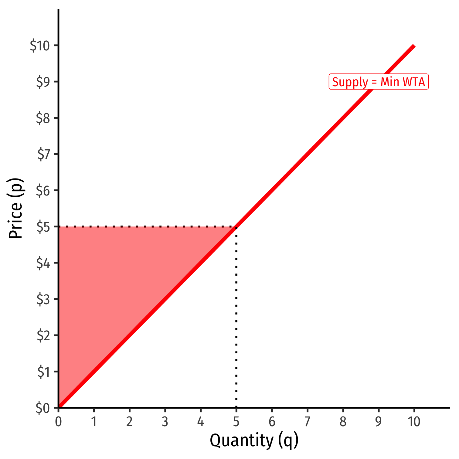
Producer Surplus II
PS=12bhPS=12(5−0)($5−$0)PS=$12.50

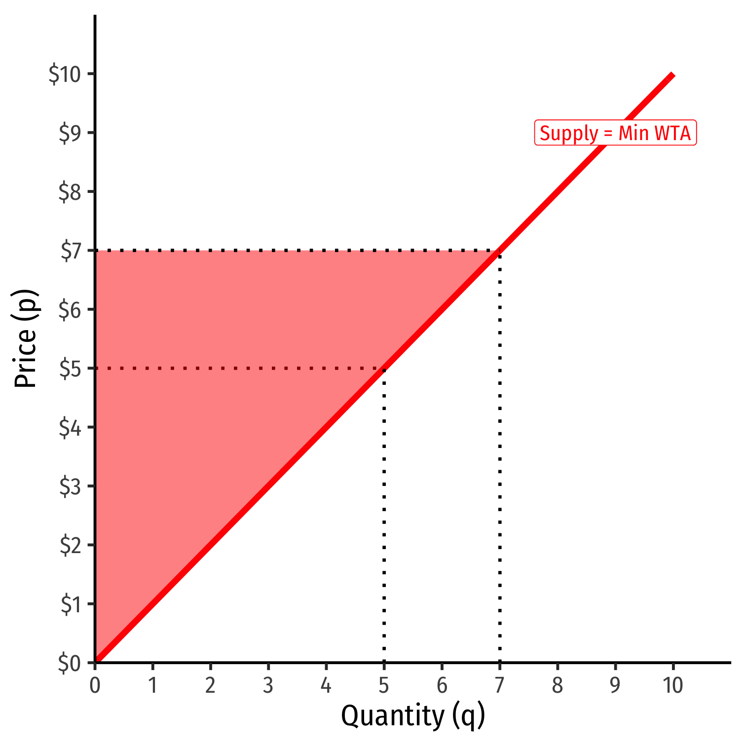
Producer Surplus III
- An increase in market price increses producer surplus
PS′=12bhPS′=12(7−0)($7−$0)PS′=$24.50
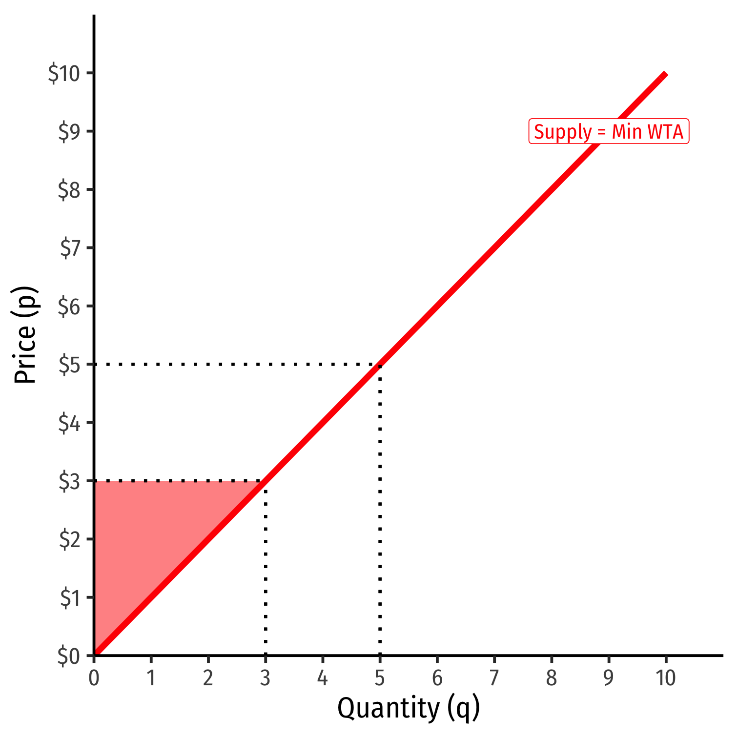
Producer Surplus IV
- An decrease in market price decreases producer surplus
PS′=12bhPS′=12(3−0)($3−$0)PS′=$4.50
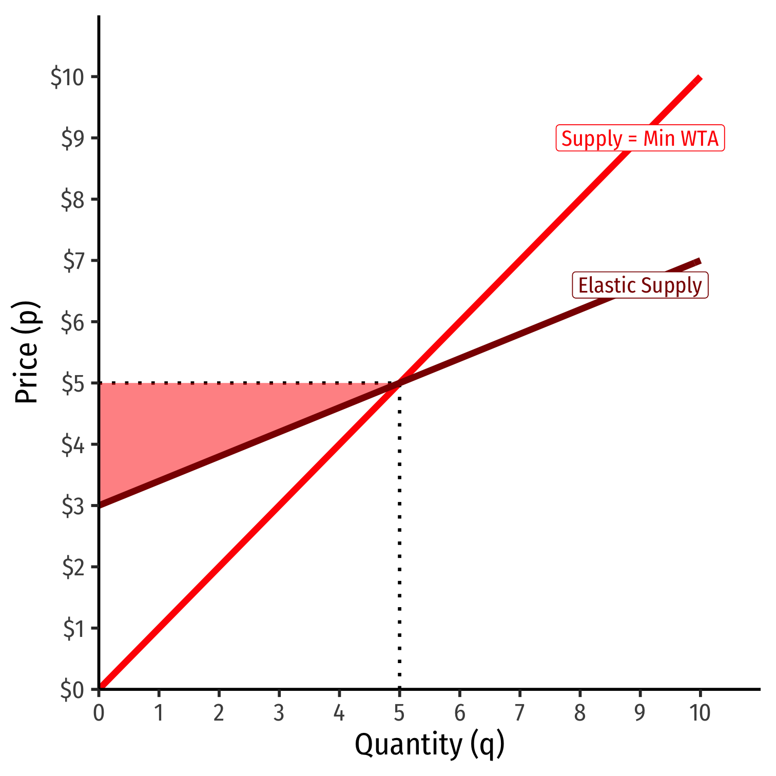
Producer Surplus V
- A relatively inelastic supply curve generates more producer surplus
PS=12bhPS=12(5−0)($5−$0)PS=$12.50
Producer Surplus V
- A relatively inelastic supply curve generates more producer surplus
PS=12bhPS=12(5−0)($5−$0)PS=$12.50
- A relatively elastic supply curve generates less producer surplus
PS=12bhPS=12(5−0)($5−$3)PS=$5.00
Elasticities and Surpluses I
The more elastic curve at p∗ generates less surplus
- More options, easier to change choices, less benefit from any one particular exchange
The less elastic curve at p∗ generates more surplus
- Fewer options, harder to change choices, more benefit from any one particular exchange
This is important for policies such as price controls, taxes, etc.
Elasticities and Surpluses II
A good visual rule of thumb:
Compare distance between choke price and p∗ for each curve
Bigger distance ⟹ less elastic in equilibrium (and vice versa)
- ⟹ more surplus