Recall: The Two Major Models of Economics as a "Science"
Optimization
Agents have objectives they value
Agents face constraints
Make tradeoffs to maximize objectives within constraints

Recall: The Two Major Models of Economics as a "Science"
Optimization
Agents have objectives they value
Agents face constraints
Make tradeoffs to maximize objectives within constraints
Equilibrium
Agents face competition from others that affect prices
Agents adjust their behaviors based on prices
Stable outcomes result where all agents cease adjusting

Recall: Optimization and Equilibrium
If people can learn and change their behavior, they will always switch to a higher-valued option
If there are no alternatives that are better, people are at an optimum
If everyone is at an optimum, the system is in equilibrium

Equilibrium Analysis: Questions to Answer
Where do prices come from?
How do they change?
How consumers and producers to respond to changes?

Equilibrium Analysis
An equilibrium is an allocation of resources such that no individual has an incentive to alter their behavior
In markets: "market-clearing" prices where quantity supplied equals quantity demanded
Partial Equilibrium Analysis
We will only look at "partial equilibrium" in a single market
Changes in one market often affect other markets, affecting the "general equilibrium"
- e.g. a change in the price of corn will affect the market for wheat, soybeans, flax, cereal, sugar, candy, ethanol, gasoline, automobiles, etc...
- think of all of the complements, substitutes, upstream and downstream goods in production...
- General equilibrium is too complicated for undergraduate courses...
Demand Curve
Demand curve graphically represents the demand schedule
Also measures a person's maximum willingness to pay (WTP) for a given quantity
Law of Demand (price effect) ⟹ Demand curves always slope downwards
Demand Function
- Demand function relates quantity to price
Example: q=10−p
- Not graphable (wrong axes)!

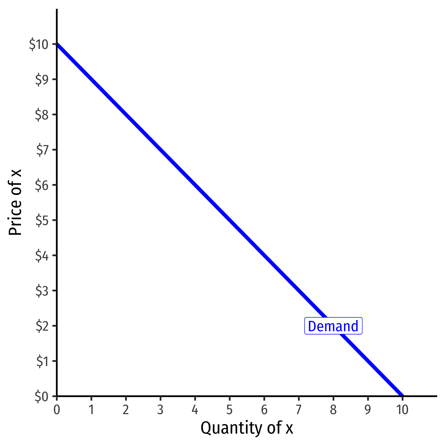
Inverse Demand Function
- Inverse demand function relates price to quantity
- Find by taking demand function and solving for p
Example: p=10−q
Graphable (price on vertical axis)!
Slope: −1
Vertical intercept called the "Choke price": price where qD=0 ($10), just high enough to discourage any purchases

Inverse Demand Function
- Inverse demand function relates price to quantity
- Find by taking demand function and solving for p
Example: p=10−q
Read two ways:
Horizontally: at any given price, how many units person wants to buy
Vertically: at any given quantity, the maximum willingness to pay (WTP) for that quantity
- This way will be very useful later

Supply Function
- Supply function relates quantity supplied to price
Example: q=2p−8
- Not graphable (wrong axes)!

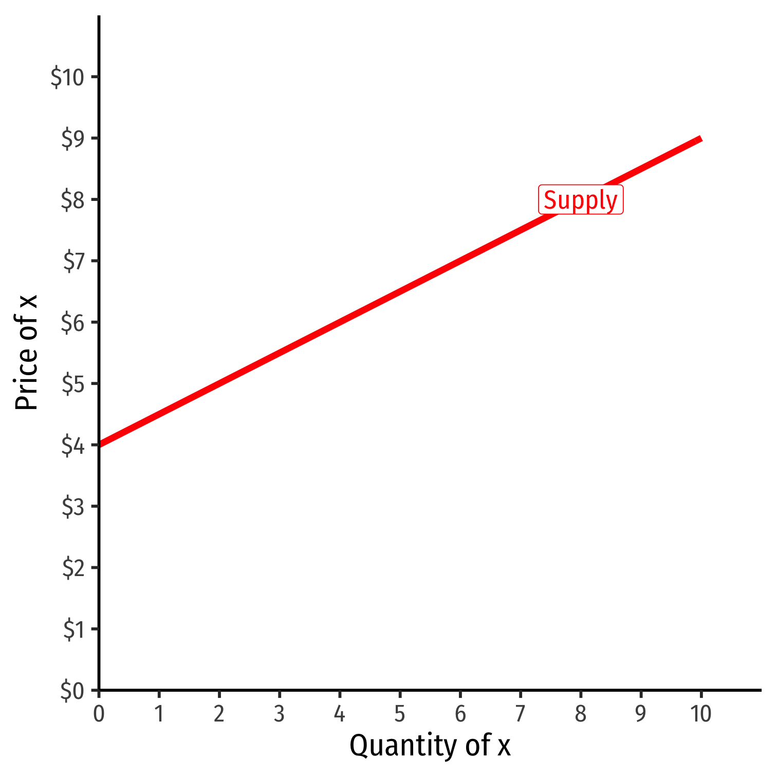
Inverse Supply Function
- Inverse supply function relates price to quantity
- Find by taking supply function and solving for p
Example: p=4+0.5q
Graphable (price on vertical axis)!
Slope: 0.5
Vertical intercept called the "Choke price": price where qS=0 ($4), just low enough to discourage any sales
Inverse Supply Function
- Inverse supply function relates price to quantity
- Find by taking suuply function and solving for p
Example: p=4+0.5q
Read two ways:
Horizontally: at any given price, how many units firm wants to sell
Vertically: at any given quantity, the minimum willingness to accept (WTA) for that quantity

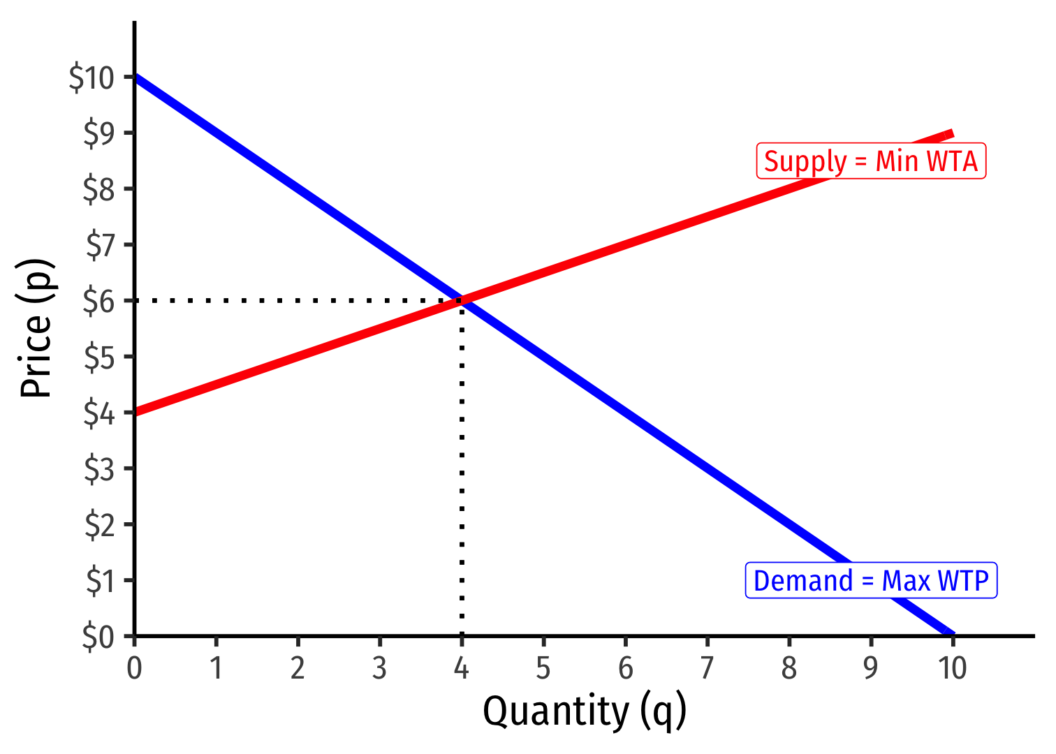
Market Equilibrium
Market-clearing (equilibrium) price (p∗): $6.00
Market-clearing (equilibrium) quantity exchanged (q∗): 4

Calculating Equilibrium: Example I
Example: Take our example supply and demand functions:
qd=10−pqs=2p−8
- In equilibrium: quantity demanded equals quantity supplied