Firm Decisions in the Long Run I
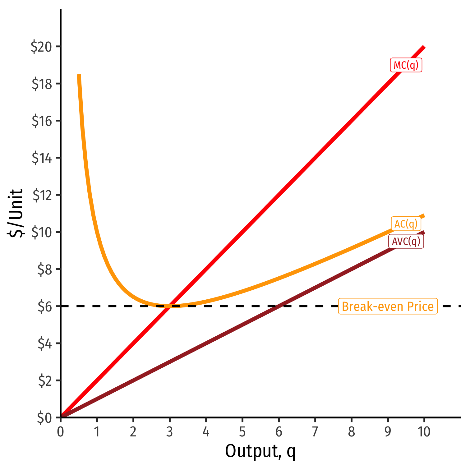
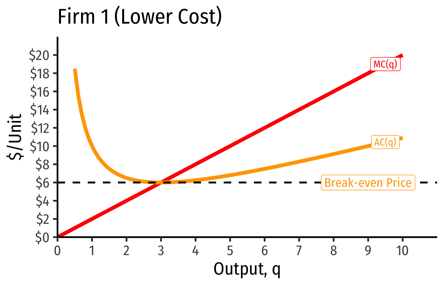
AC(q)min happens at a market price of $6.00
At $6.00, the firm earns "normal economic profits" of 0.
At any market price below $6.00, firm earns losses
- In the Short Run: firm shuts down production only if p<AVC(q)
At any market price above $6.00, firm earns "supernormal profits"
Firm Supply Decisions in the Short Run vs. Long Run
Short run: firms that shut down (q∗=0) stuck in market, incur fixed costs π=−f
- Firms cannot change their fixed factor (capital k)
Long run: firms earning losses (π<0) can exit the market and earn π=0
- No more fixed costs, firms can sell/abandon f at q∗=0
Entrepreneurs & Firms not currently in market can choose to enter and start producing, if entry would earn them π>0

Firm's Long Run Supply: Visualizing
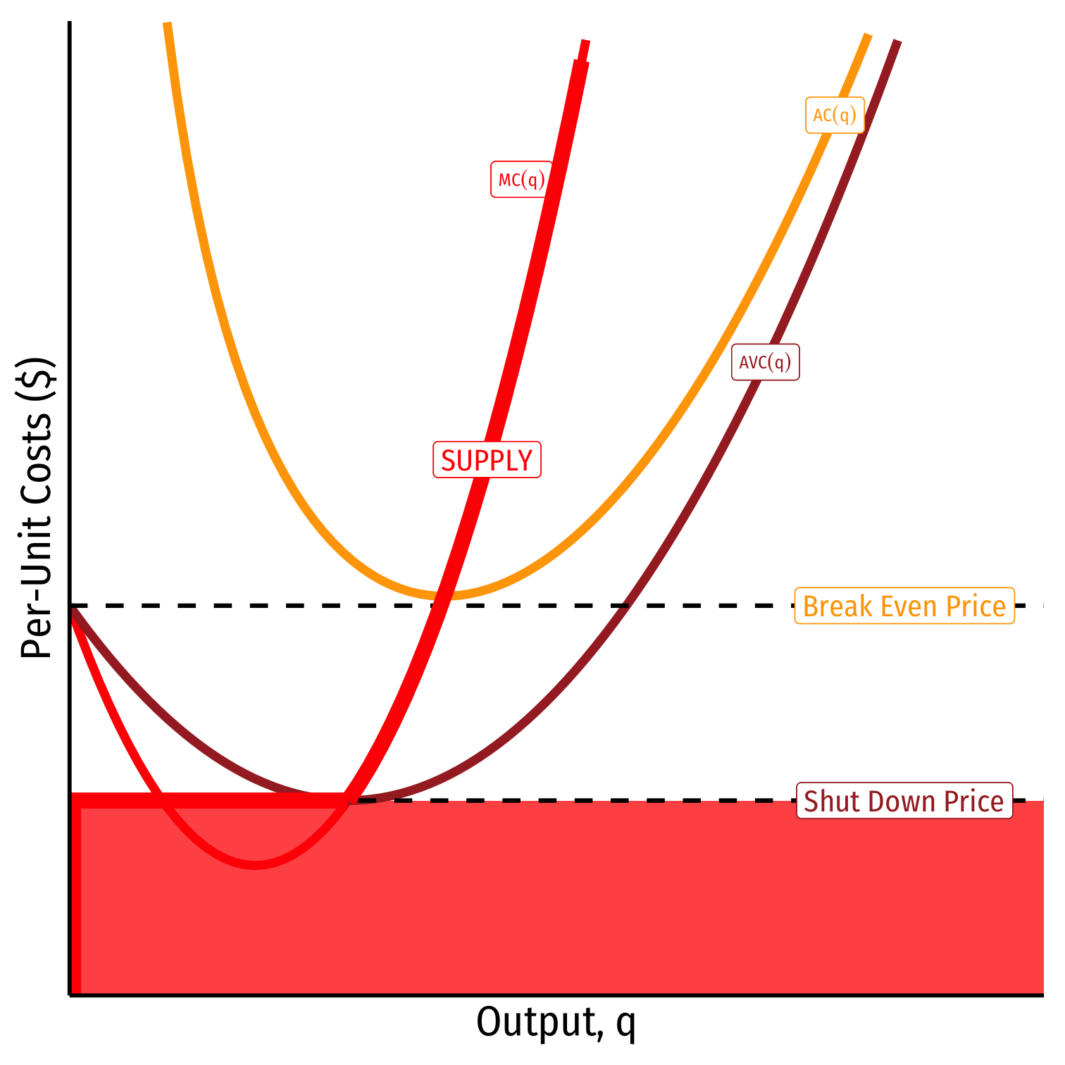
When p<AVC
Profits are negative
Short run: shut down production
- Firm loses more π by producing than by not producing
Long run: firms in industry exit the industry
- No new firms will enter this industry
Firm's Long Run Supply: Visualizing
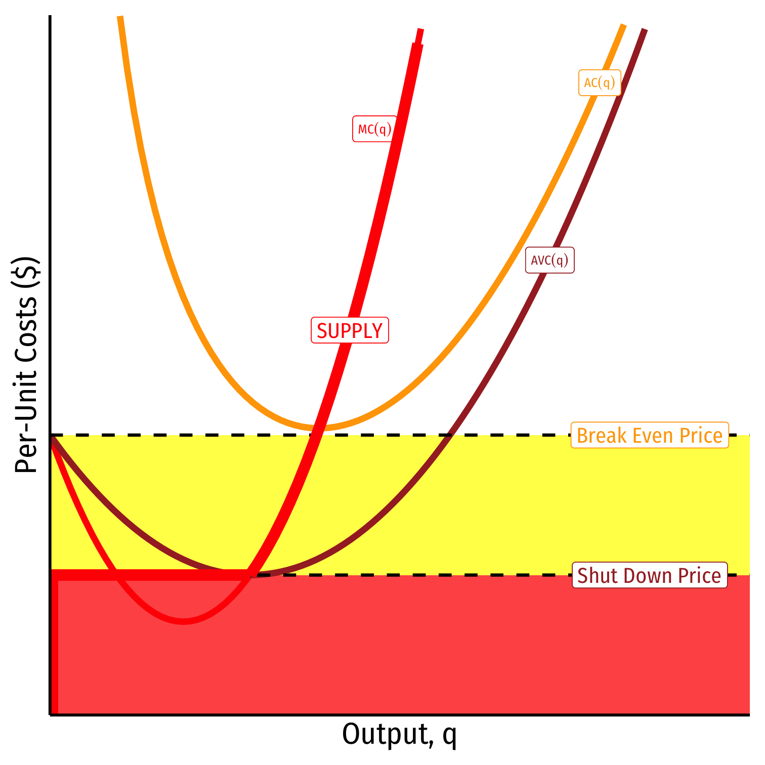
When AVC<p<AC
Profits are negative
Short run: continue production
- Firm loses less π by producing than by not producing
Long run: firms in industry exit the industry
- No new firms will enter this industry
Firm's Long Run Supply: Visualizing
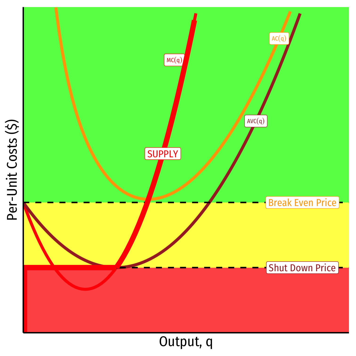
When AC<p
Profits are positive
Short run: continue production
- Firm earn profits
Long run: firms in industry stay in industry
- New new firms will enter this industry
Recall: The Two Major Models of Economics as a "Science"
Optimization
Agents have objectives they value
Agents face constraints
Make tradeoffs to maximize objectives within constraints

Recall: The Two Major Models of Economics as a "Science"
Optimization
Agents have objectives they value
Agents face constraints
Make tradeoffs to maximize objectives within constraints
Equilibrium
Agents face competition from others that affect prices
Agents adjust their behaviors based on prices
Stable outcomes result where all agents cease adjusting

Recall: Optimization and Equilibrium
If people can learn and change their behavior, they will always switch to a higher-valued option
If there are no alternatives that are better, people are at an optimum
If everyone is at an optimum, the system is in equilibrium

Exit, Entry, and Long Run Industry Equilibrium I
Now we must combine optimizing individual firms with market-wide adjustment to equilibrium
Since π=[p−AC(q)]q, in the long run, profit-seeking firms will:
- Enter markets where p>AC(q)
Exit, Entry, and Long Run Industry Equilibrium I
Now we must combine optimizing individual firms with market-wide adjustment to equilibrium
Since π=[p−AC(q)]q, in the long run, profit-seeking firms will:
- Enter markets where p>AC(q)
- Exit markets where p<AC(q)
Exit, Entry, and Long Run Industry Equilibrium II
- Long-run equilibrium: entry and exist cases when p=AC(q) for all firms, implying normal economic profits of π=0

Exit, Entry, and Long Run Industry Equilibrium II
Long-run equilibrium: entry and exist cases when p=AC(q) for all firms, implying normal economic profits of π=0
Zero Profits Theorem: long run economic profits for all firms in a competitive industry are 0
Firms must earn an accounting profit to stay in business
A constant tendency as output prices are pushed down and input prices are bid up, squeezing economic profits to 0
In real life, constant changes in underlying prices, technology, preferences
Industry Supply Curves (Identical Firms)

Industry Supply Curves (Identical Firms)
- Industry supply curve is the horizontal sum of all individual firm's supply curves
- Which are each firm's marginal cost curve above its breakeven price
Industry Supply Curves (Identical Firms)

- Industry demand curve (where equal to supply curve) sets market price, demand for each firm
Industry Supply Curves (Identical Firms)


Industry demand curve (where equal to supply curve) sets market price, demand for each firm
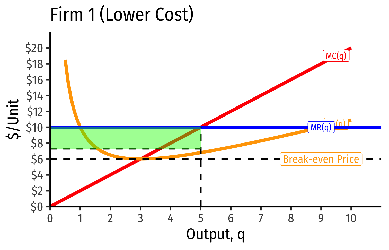
Short Run: each firm is earning profits p>AC(q)
Long run: induces entry by firm 3, firm 4, ⋯, firm n
Industry Supply Curves (Identical Firms)
Industry demand curve (where equal to supply curve) sets market price, demand for each firm
Short Run: each firm is earning profits p>AC(q)
Long run: induces entry by firm 3, firm 4, ⋯, firm n
Long run industry equilibrium:
Industry Supply Curves (Identical Firms)
Industry demand curve (where equal to supply curve) sets market price, demand for each firm
Short Run: each firm is earning profits p>AC(q)
Long run: induces entry by firm 3, firm 4, ⋯, firm n
Long run industry equilibrium: p=AC(q)min, π=0 at p= $6
- Supply becomes more elastic (more firms supplying more output)
Industry Supply Curves (Different Firms) I
- Firms may have different cost structures due to differences in:
- Managerial talent
- Worker talent
- Location
- First-mover advantage
- Technological secrets/IP
- License/permit access
- Political connections
- Lobbying

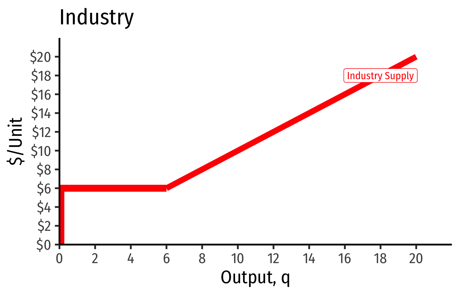
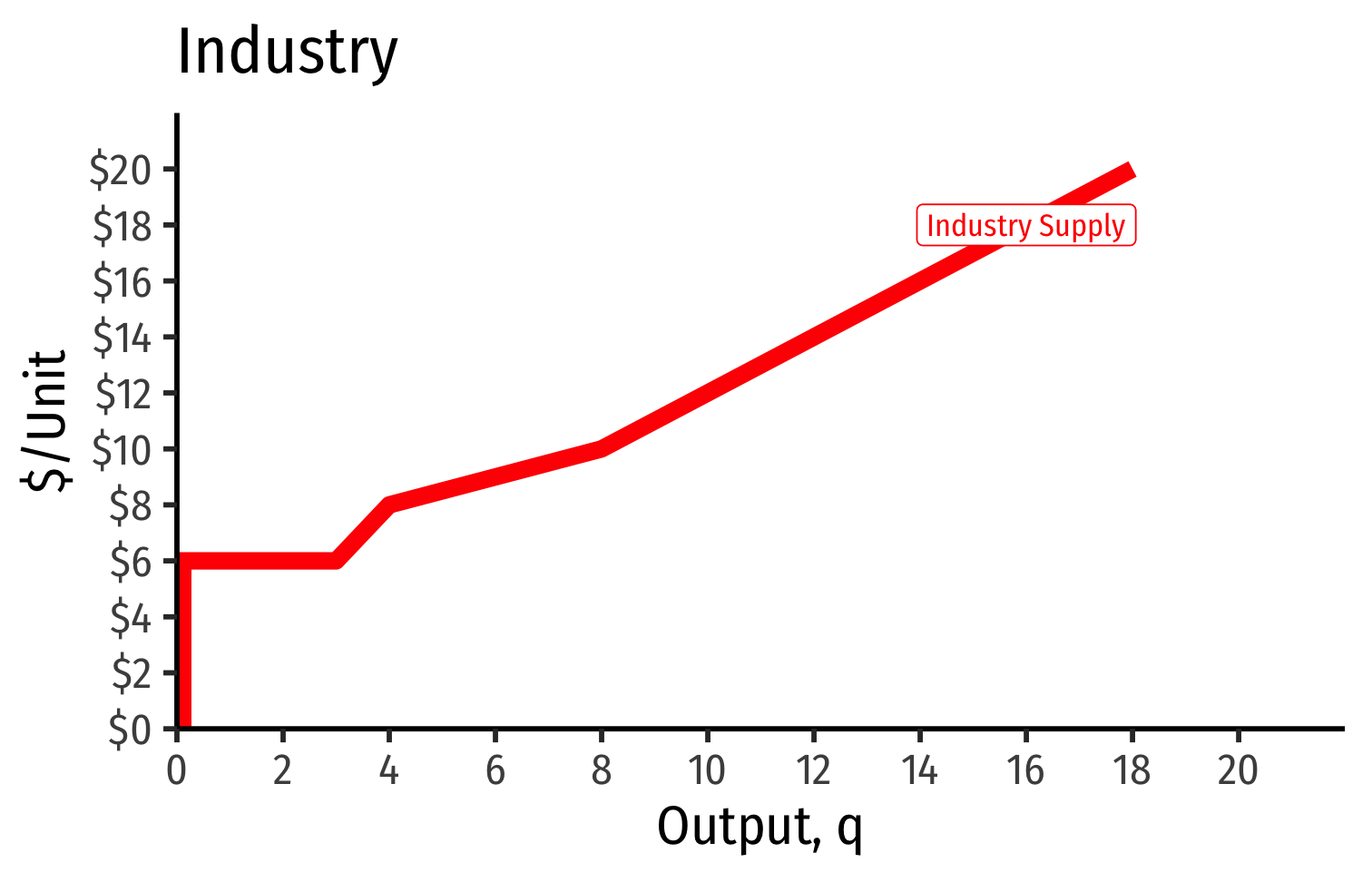
Industry Supply Curves (Different Firms) II
Industry Supply Curves (Different Firms) II
- Industry supply curve is the horizontal sum of all individual firm's supply curves
- Which are each firm's marginal cost curve above its breakeven price
Industry Supply Curves (Different Firms) II
Industry Supply Curves (Different Firms) II
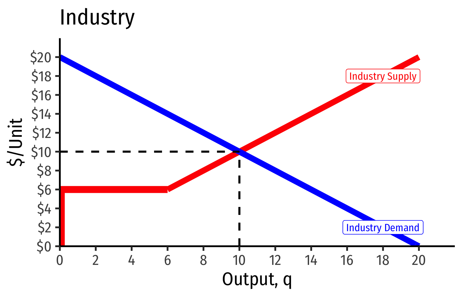
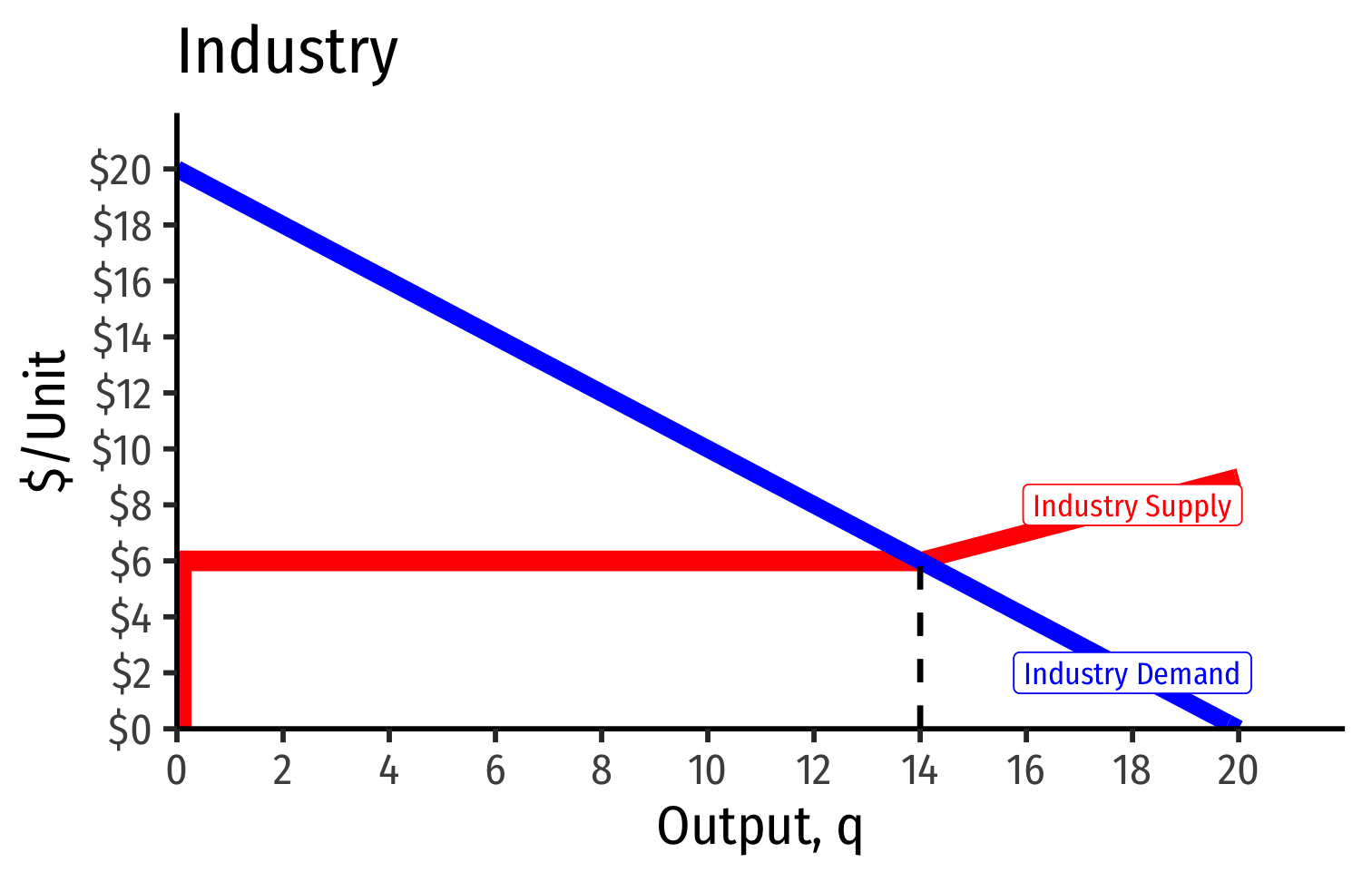
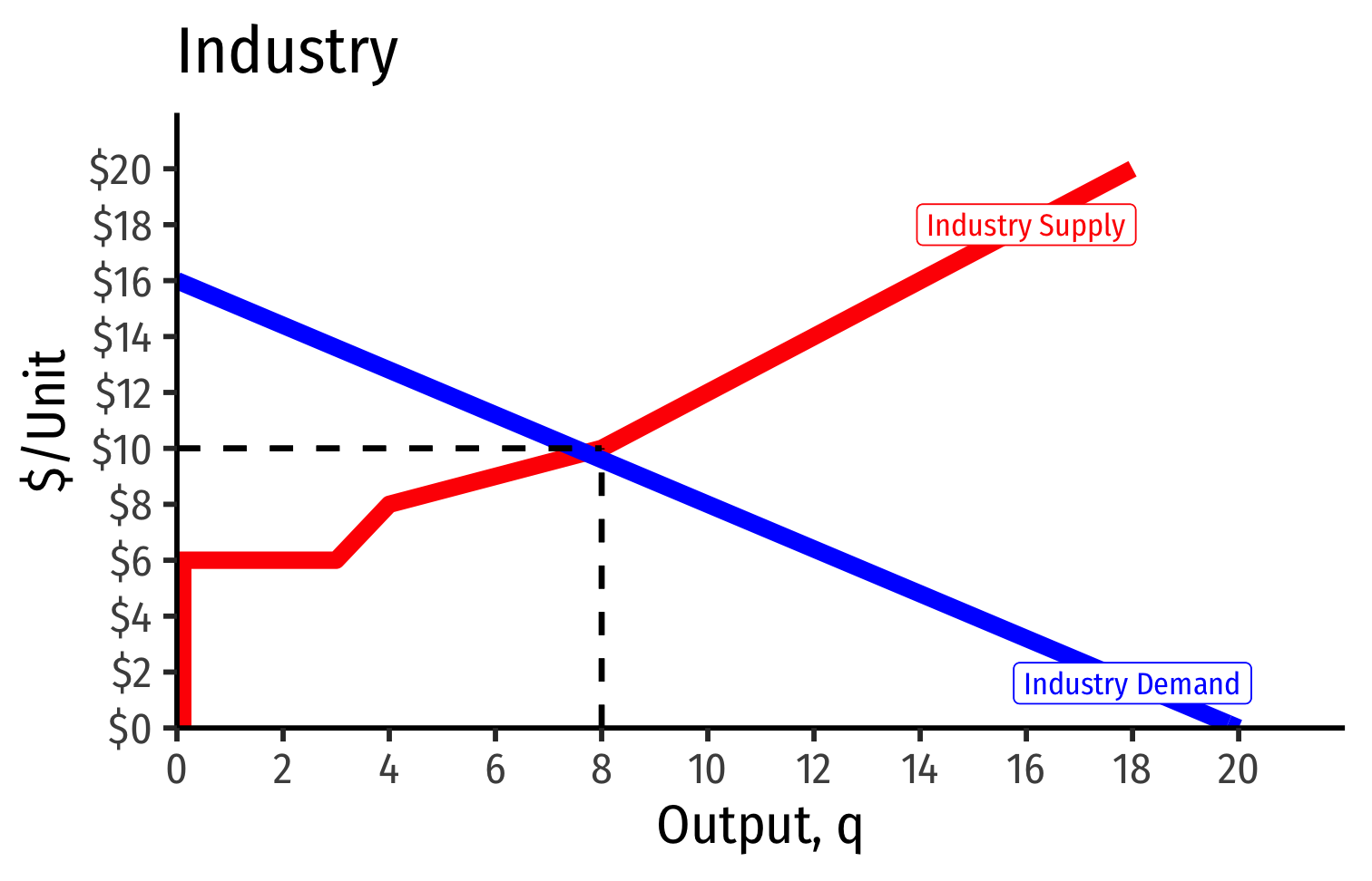
- Industry demand curve (where equal to supply curve) sets market price, demand for each firm
Industry Supply Curves (Different Firms) II
Industry demand curve (where equal to supply curve) sets market price, demand for each firm
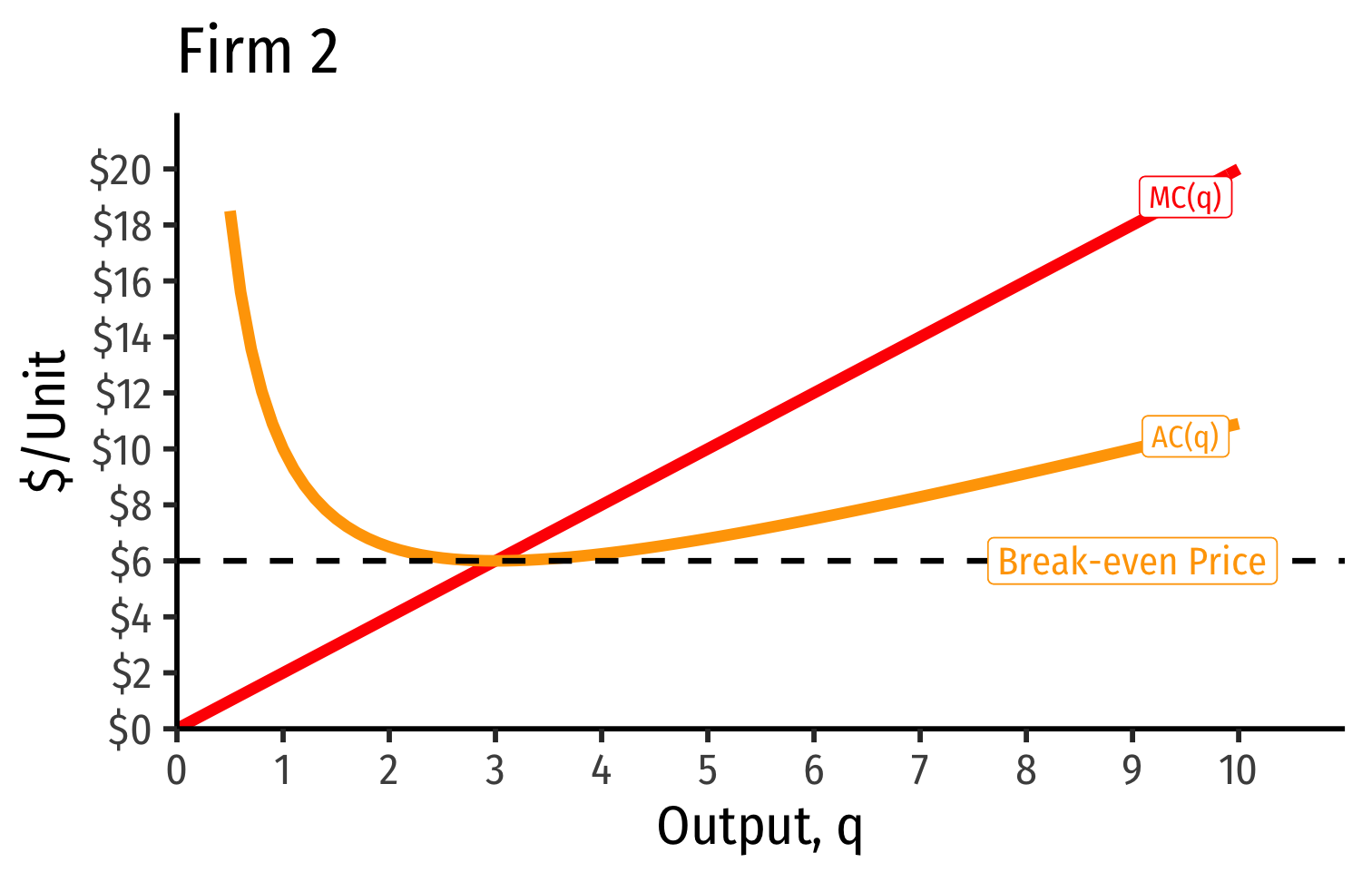
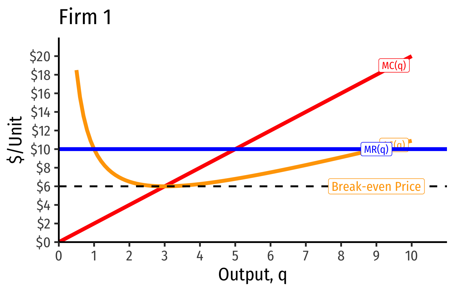
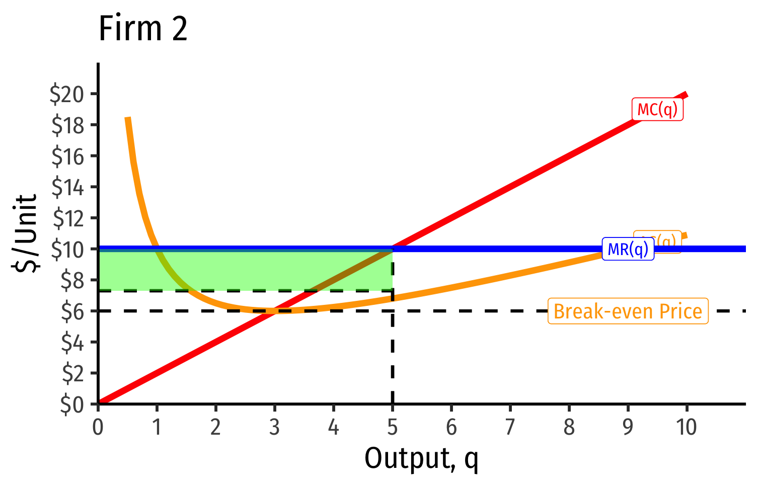
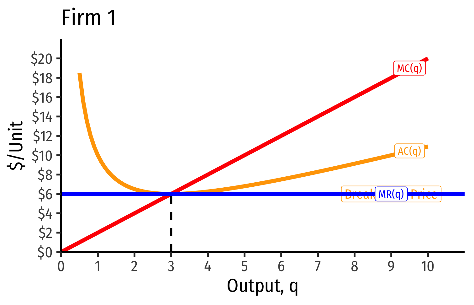
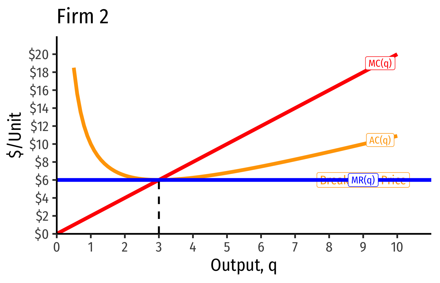
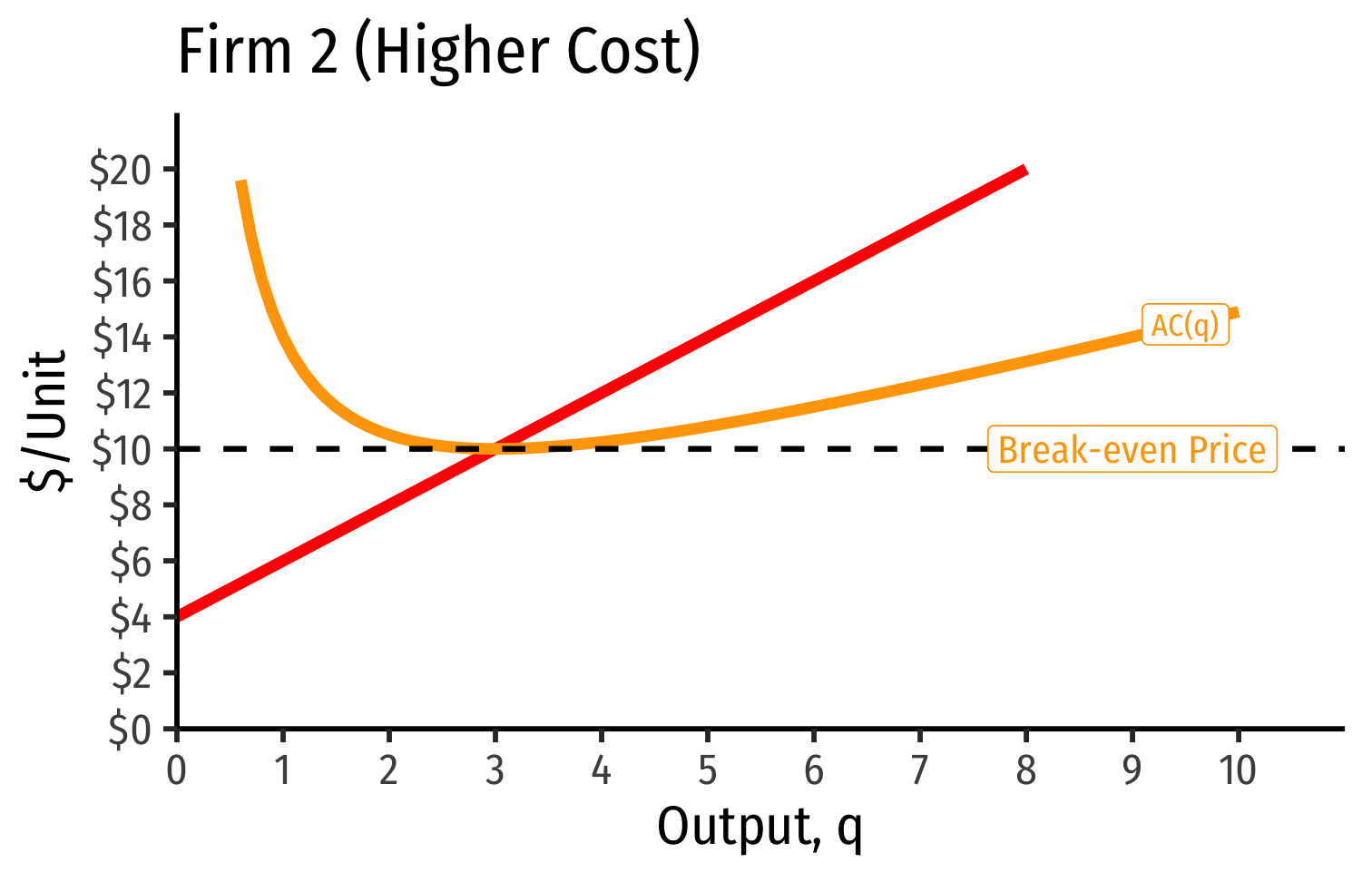
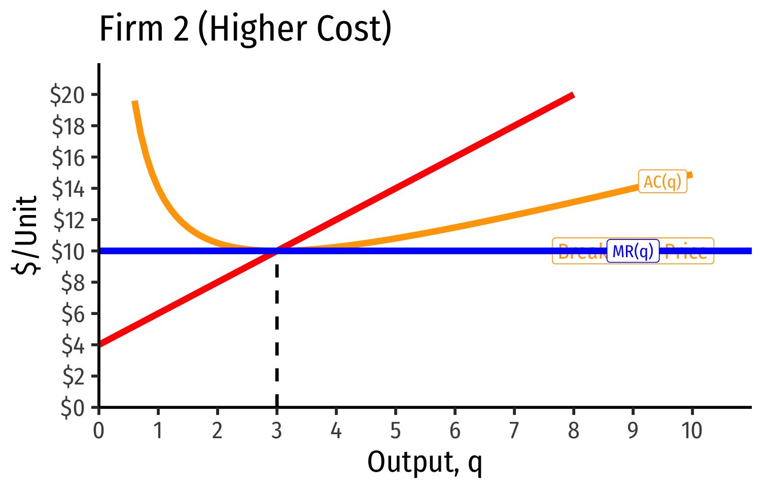
Long run industry equilibrium: p=AC(q)min, π=0 for marginal (highest cost) firm (Firm 2)
Industry Supply Curves (Different Firms) II
Industry demand curve (where equal to supply curve) sets market price, demand for each firm
Long run industry equilibrium: p=AC(q)min, π=0 for marginal (highest cost) firm (Firm 2)
Firm 1 (lower cost) appears to be earning profits
Economic Rents and Zero Economic Profits I

With differences between firms, long-run equilibrium p=AC(q)min of the marginal (highest-cost) firm
- If p>AC(q) for that firm, would induce more entry into industry!
"Inframarginal" (lower-cost) firms earn economic rents: returns higher than their opportunity cost (what is needed to bring them online
- p>AC(q)
Economic rents arise from relative differences between firms
Economic Rents and Zero Economic Profits II
Relatively scarce factors in the economy (talent, location, secrets, IP, licenses, being first, political favoritism, lobbying)
Inframarginal firms using the scarce factors gain a cost-advantage
It would seem these firms earn profits as other firms have higher costs
But what will happen to the prices for the scarce factors?
Rent: Microeconomics IV

Rents ≠ profits!
Rival firms willing to pay for rent-generating factor to gain advantage
Rents are included in the opportunity cost (price) for inputs
Firm does not earn the rents, they raise firm's costs and squeeze out profits!
Factor owners (workers, landowners, inventors, etc) earn the rents as higher payments for their services (wages, rents, interest, royalties, etc).
Recall: Accounting vs. Economic Point of View
- Helpful to consider two points of view:
- "Accounting point of view": are you taking in more cash than you are spending?
- "Economic point of view: is your product you making the best social use of your resources (i.e. are there higher-valued uses of your resources you are keeping them away from)?


Constant Cost Industry (No External Economies) I
Constant cost industry has no external economies, no change in costs as industry output increases (firms enter & incumbents produce more)
A perfectly elastic long-run industry supply curve!
Determinants:
- Industry's purchases are not a large share of input markets
- Often constant marginal costs, insignificant fixed costs
Examples: toothpicks, domain name registration, waitstaff


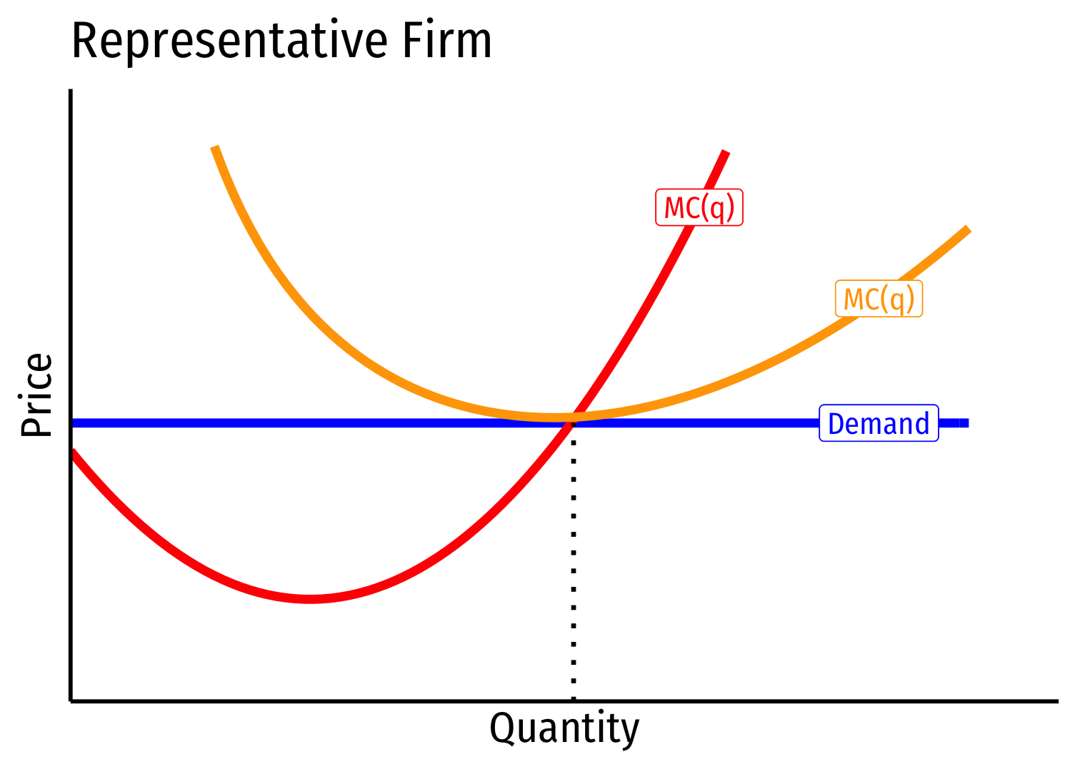
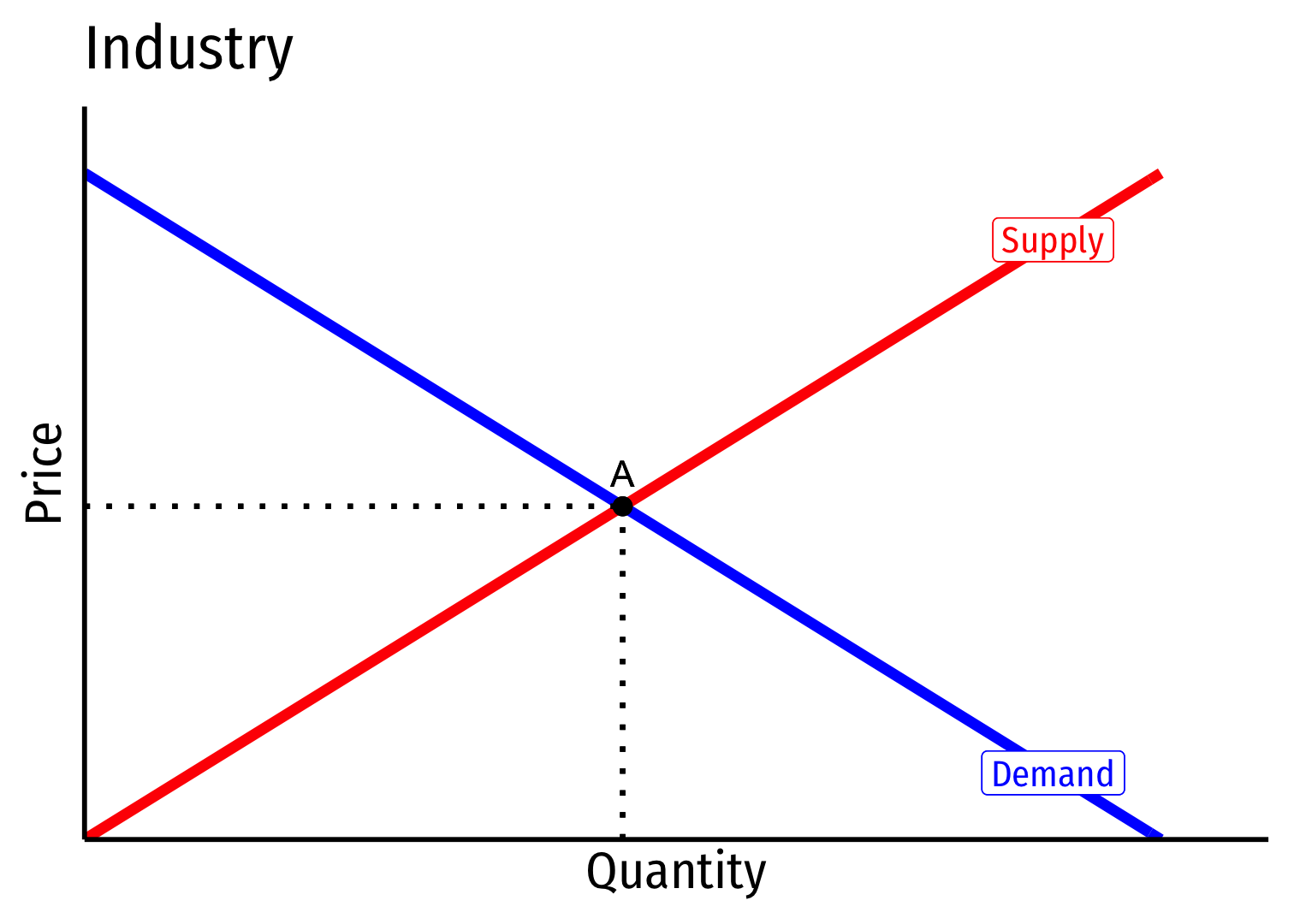
Constant Cost Industry (No External Economies) II


- Industry equilibrium: firms earning normal π=0,p=MC(q)=AC(q)
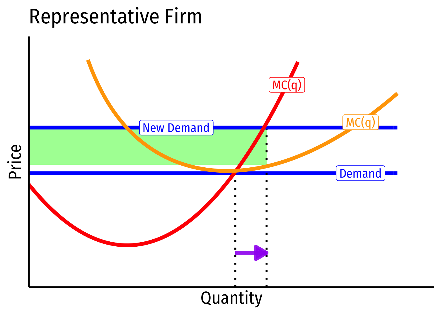
Constant Cost Industry (No External Economies) III


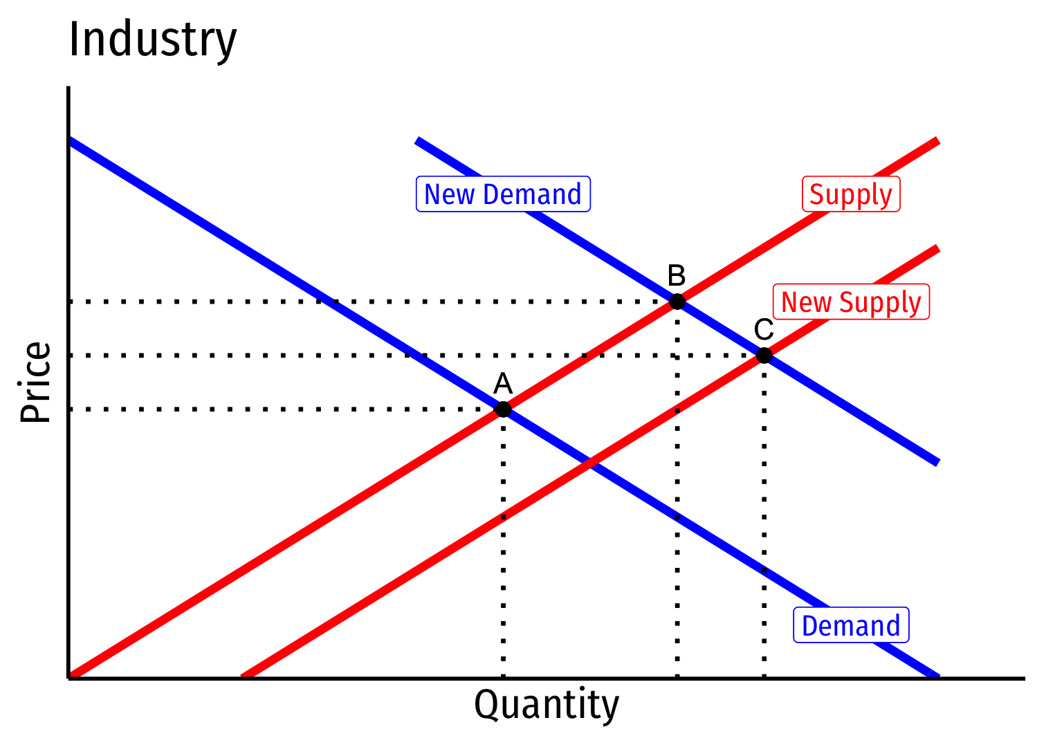
Industry equilibrium: firms earning normal π=0,p=MC(q)=AC(q)
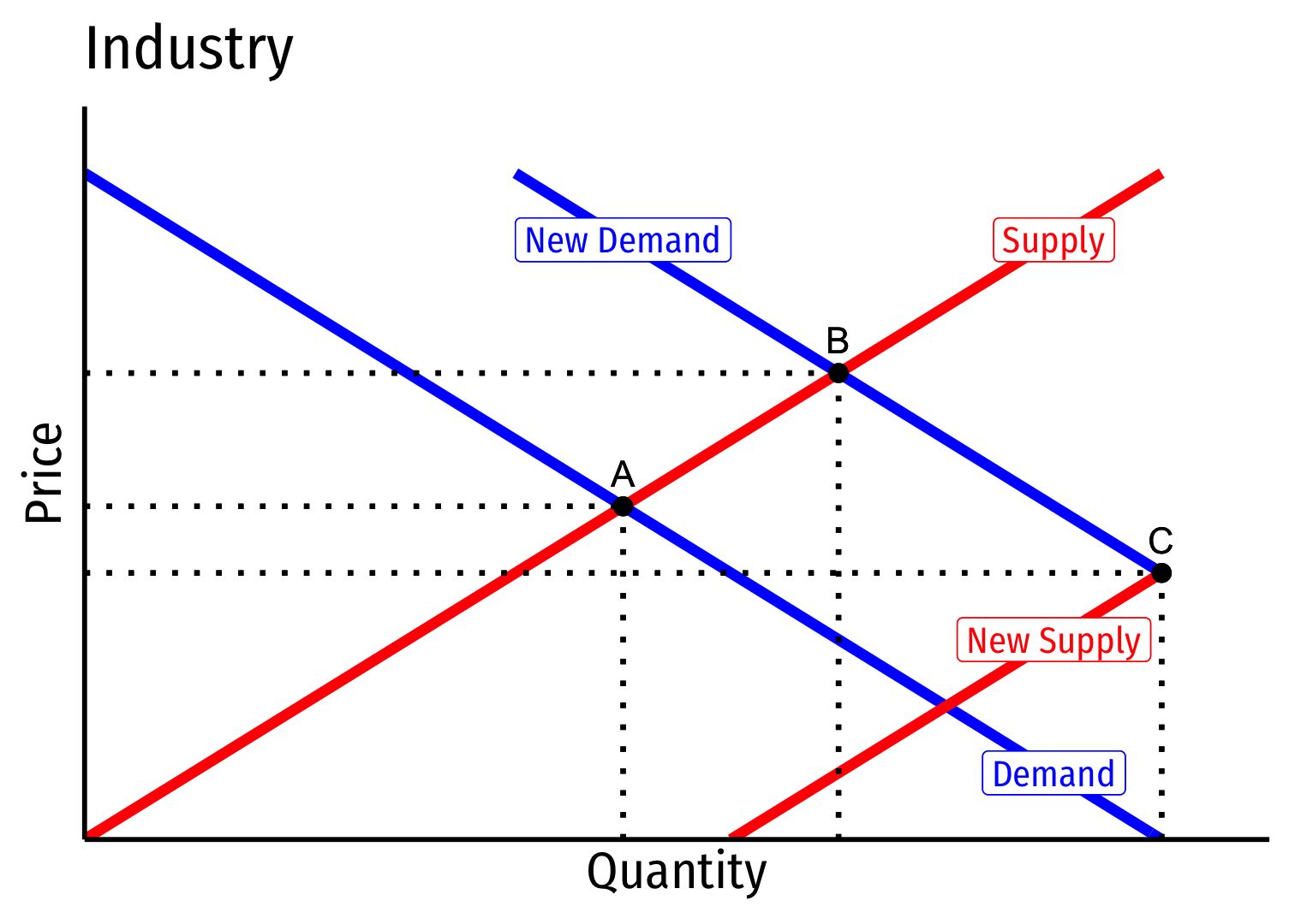
Exogenous increase in market demand
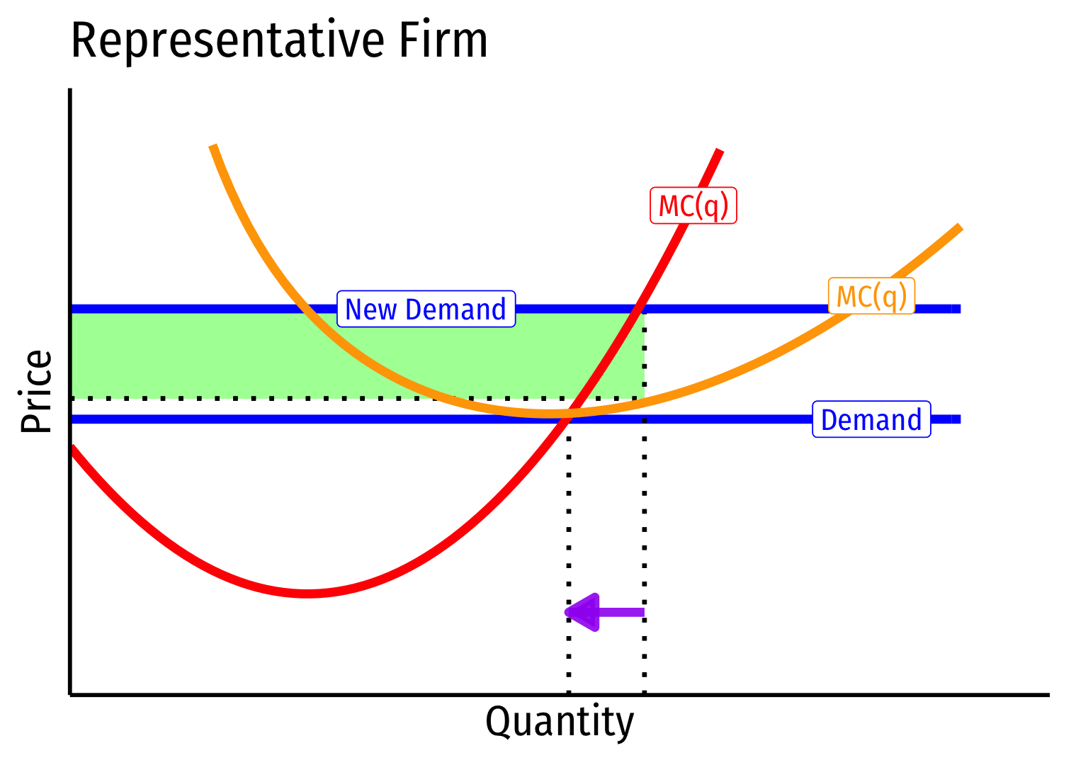
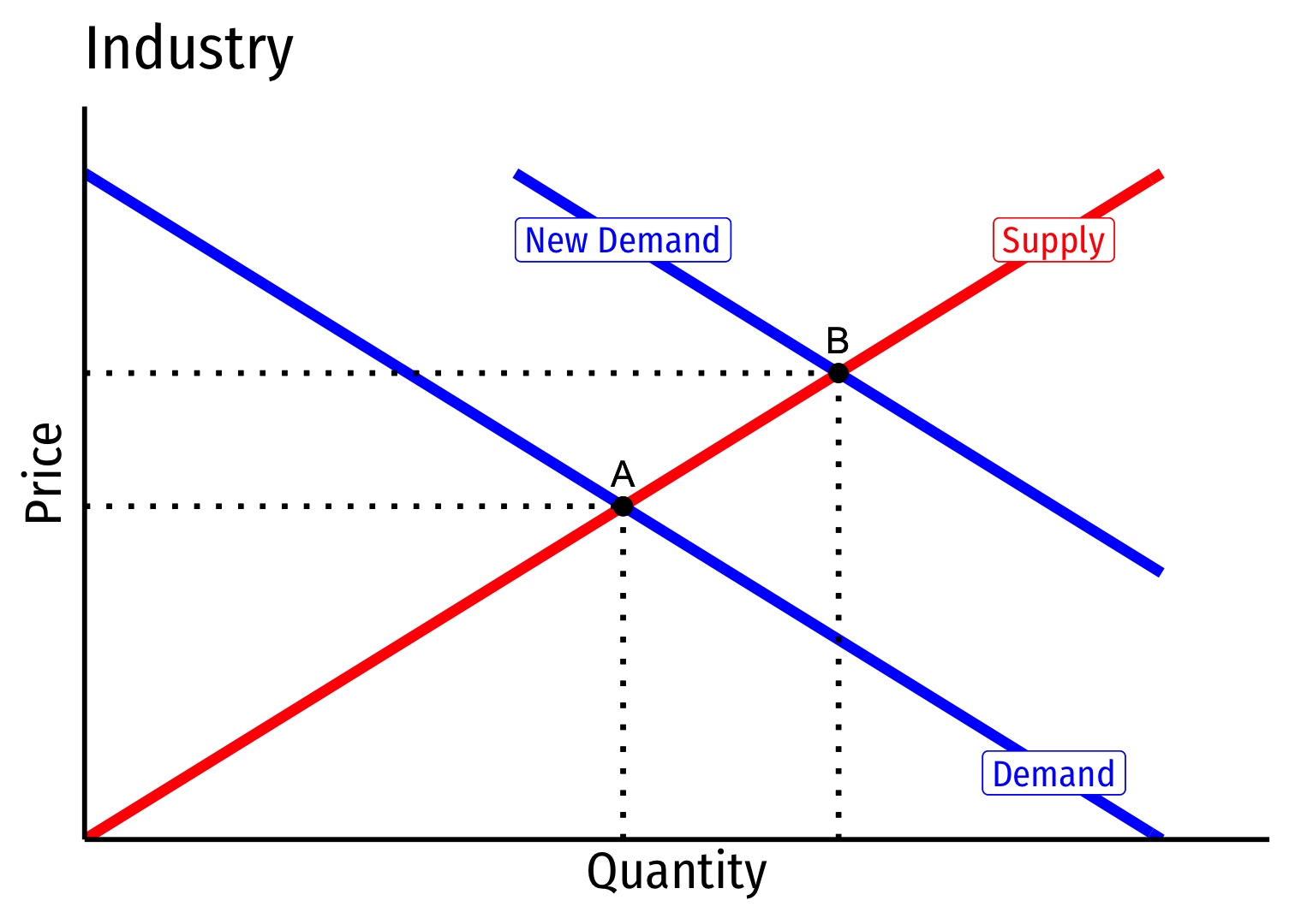
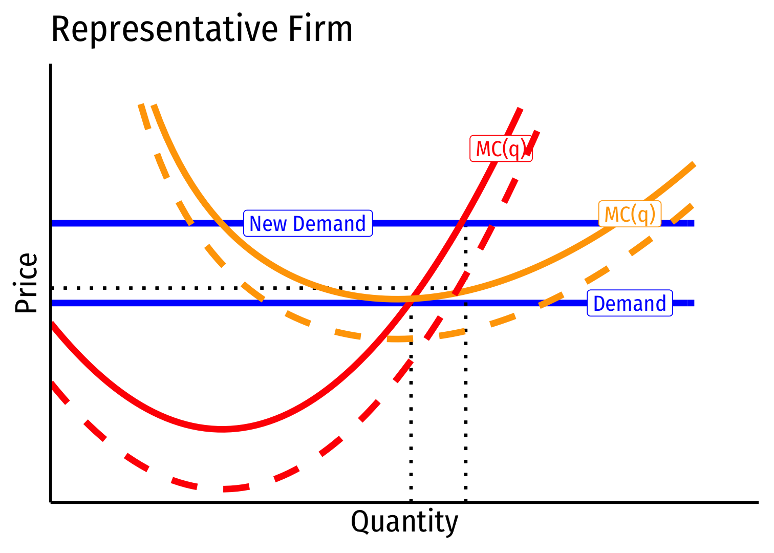
Constant Cost Industry (No External Economies) IV


Short run (A→B): industry reaches new equilibrium
Firms charge higher p∗, produce more q∗, earn π
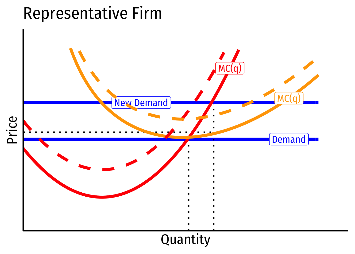
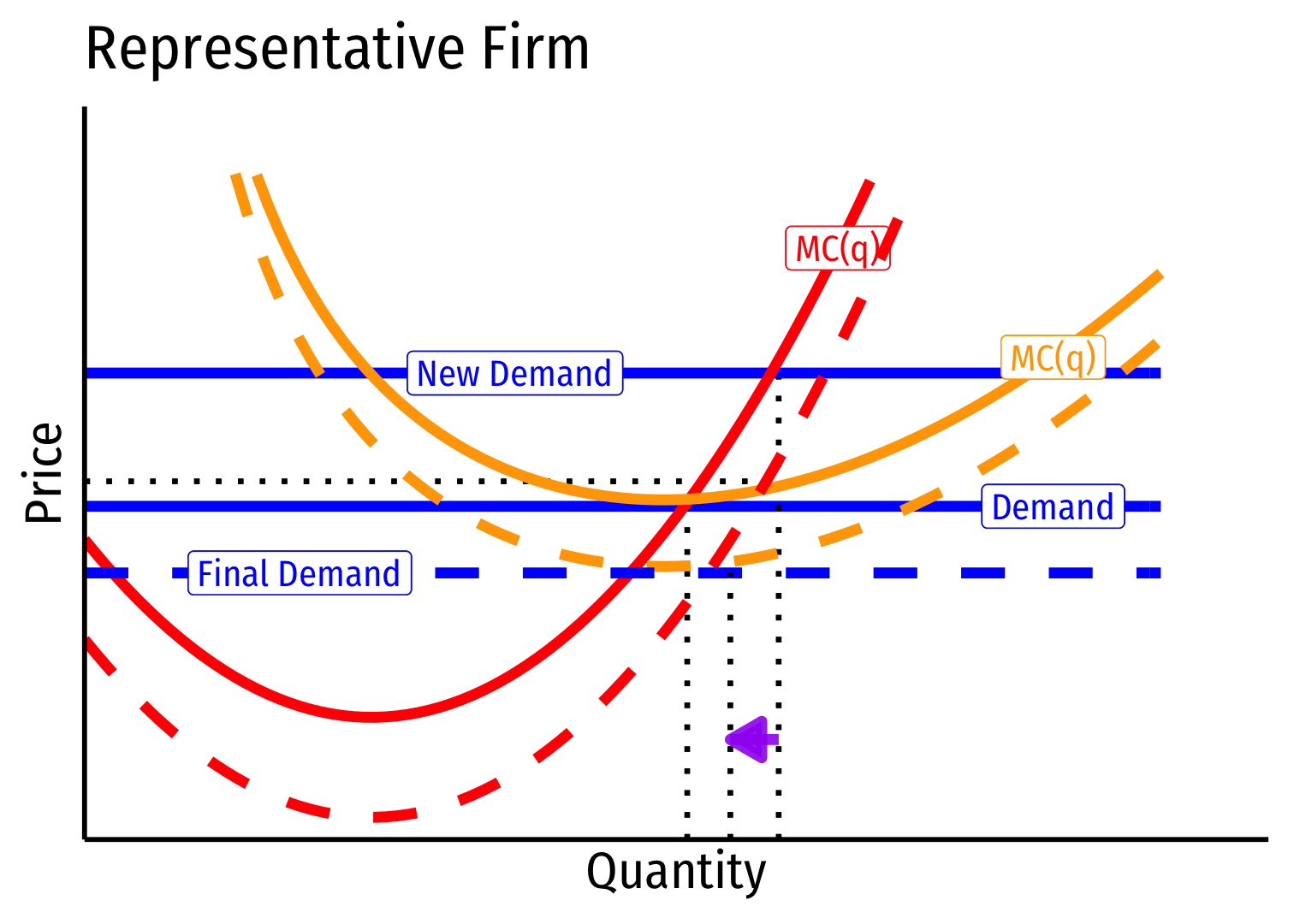
Constant Cost Industry (No External Economies) V
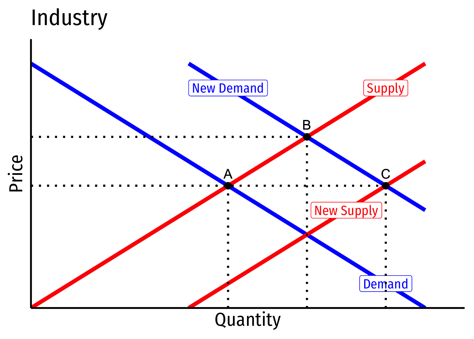
Long run (B→C): profit attracts entry ⟹ industry supply increases
No change in costs to firms in industry, firms enter until π=0 at p=AC(q)
Firms must charge original p∗, return to original q∗, earn π=0
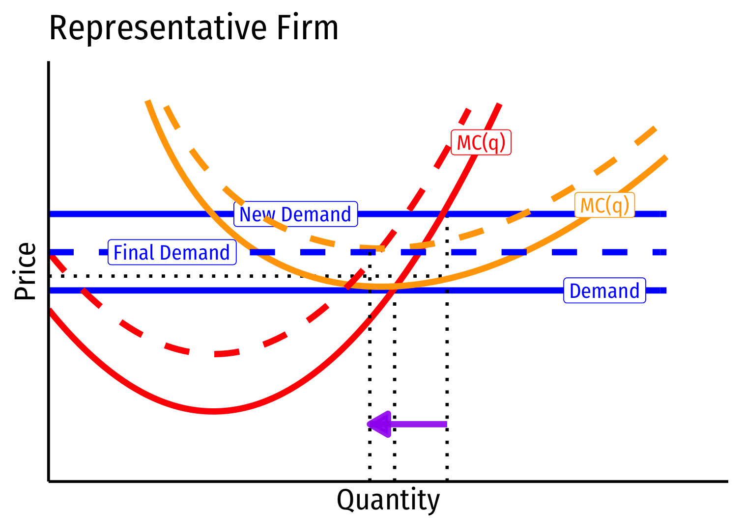
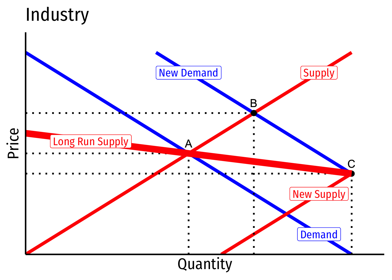
Constant Cost Industry (No External Economies) VI
- Long Run Industry Supply is perfectly elastic
Increasing Cost Industry (External Diseconomies) I
Increasing cost industry has external _dis_economies, costs rise for all firms in the industry as industry output increases (firms enter & incumbents produce more)
An upward sloping long-run industry supply curve!
Determinants:
- Finding more resources in harder-to-reach places
- Diminishing marginal products
- Greater complexity and administrative costs at larger scales
Examples: oil, mining, particle physics


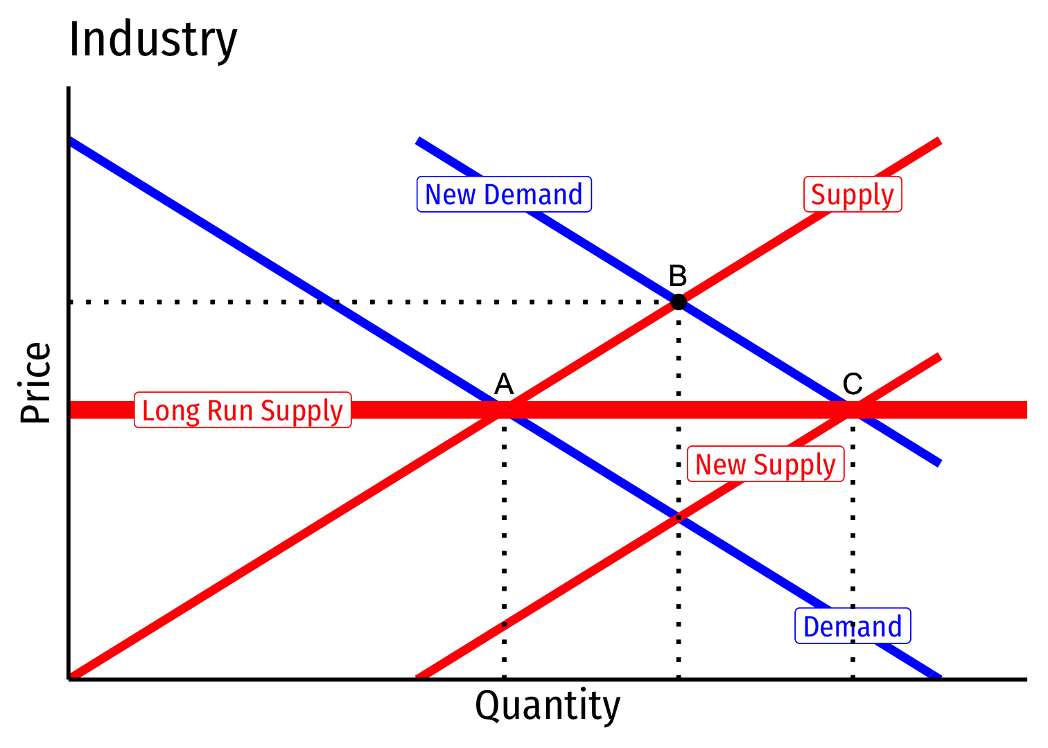
Increasing Cost Industry (External Diseconomies) II


- Industry equilibrium: firms earning normal π=0,p=MC(q)=AC(q)
Increasing Cost Industry (External Diseconomies) III
Industry equilibrium: firms earning normal π=0,p=MC(q)=AC(q)
Exogenous increase in market demand
Increasing Cost Industry (External Diseconomies) IV

Short run (A→B): industry reaches new equilibrium
Firms charge higher p∗, produce more q∗, earn π
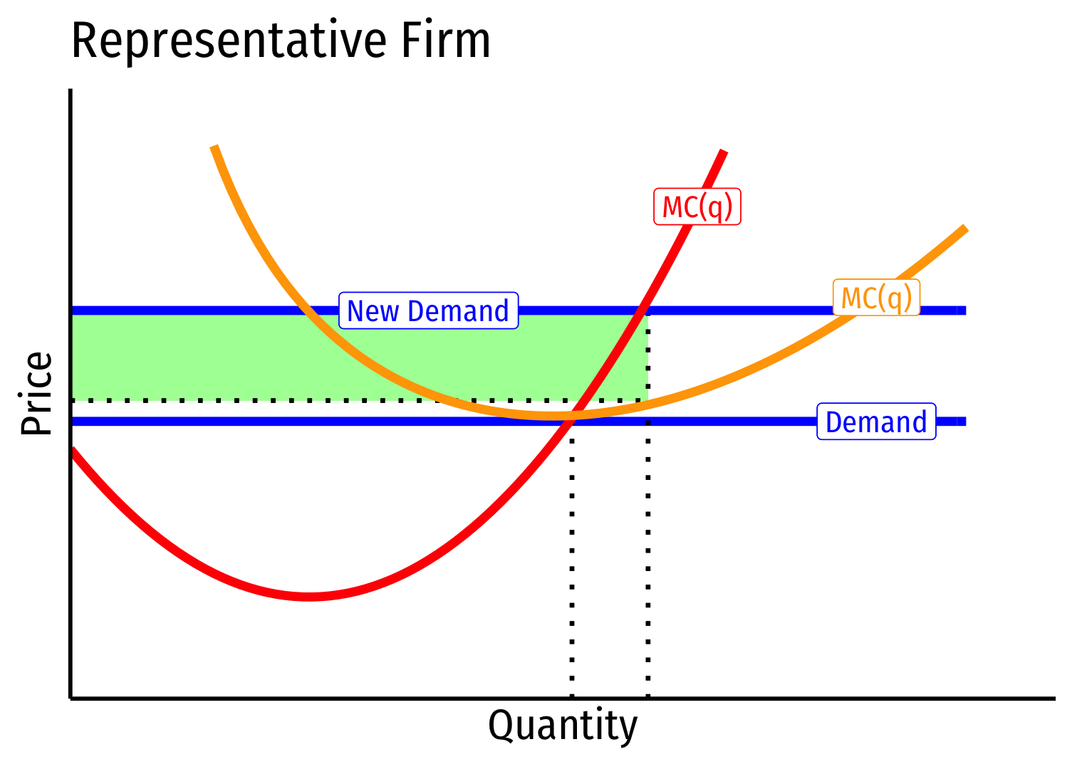
Increasing Cost Industry (External Diseconomies) V

Long run: profit attracts entry ⟹ industry supply will increase
But more production increases costs (MC,AC) for all firms in industry
Increasing Cost Industry (External Diseconomies) VI
Long run (B→C): firms enter until π=0 at p=AC(q)
Firms charge higher p∗, producer lower q∗, earn π=0
Increasing Cost Industry (External Diseconomies) VII

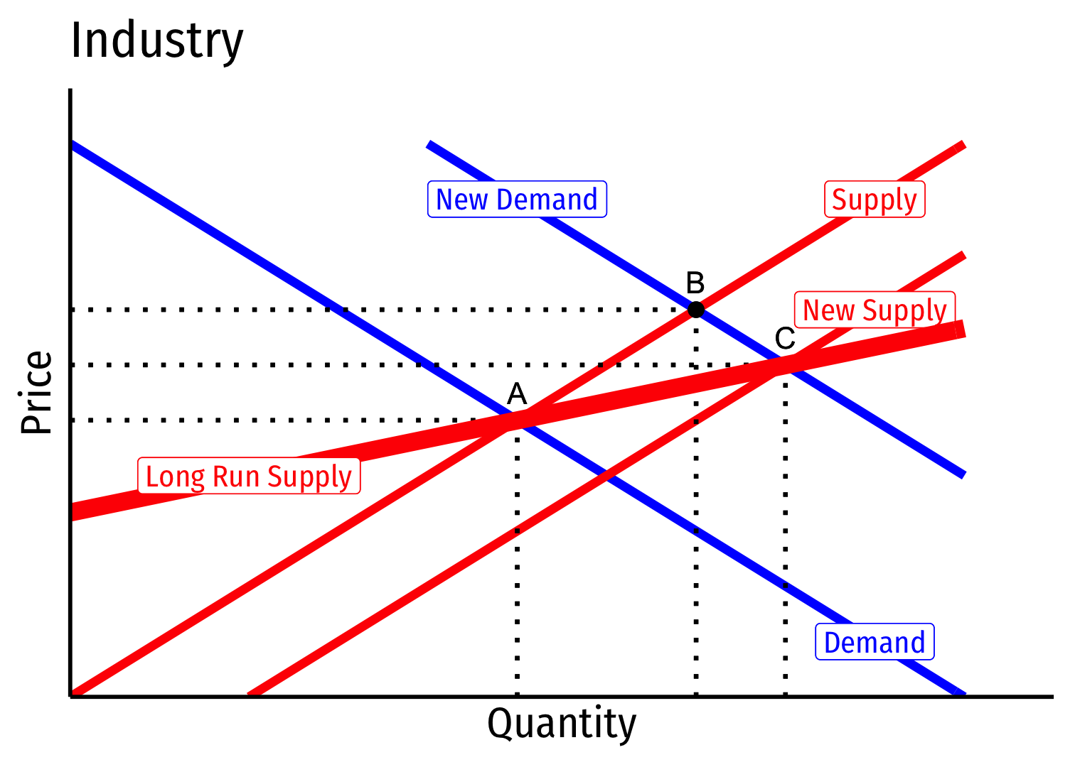
- Long run industry supply curve is upward sloping
Decreasing Cost Industry (External Economies) I
Decreasing cost industry has external economies, costs fall for all firms in the industry as industry output increases (firms enter & incumbents produce more)
A downward sloping long-run industry supply curve!
Determinants:
- High fixed costs, low marginal costs
- Economies of scale
Examples: geographic clusters, public utilities, infrastructure, entertainment
Tends towards "natural" monopoly


Decreasing Cost Industry (External Economies) II

- Industry equilibrium: firms earning normal π=0,p=MC(q)=AC(q)
Decreasing Cost Industry (External Economies) III


Industry equilibrium: firms earning normal π=0,p=MC(q)=AC(q)
Exogenous increase in market demand
Decreasing Cost Industry (External Economies) IV


Short run (A→B): industry reaches new equilibrium
Firms charge higher p∗, produce more q∗, earn π
Decreasing Cost Industry (External Economies) V

Long run: profit attracts entry ⟹ industry supply will increase
But more production lowers costs (MC,AC) for all firms in industry
Decreasing Cost Industry (External Economies) VI
Long run (B→C): firms enter until π=0 at p=AC(q)
Firms charge higher p∗, producer lower q∗, earn π=0
Decreasing Cost Industry (External Economies) VII

- Long run industry supply curve is downward sloping!
Supply Function
- Supply function relates quantity supplied to price
Example: q=2p−4
- Not graphable (wrong axes)!
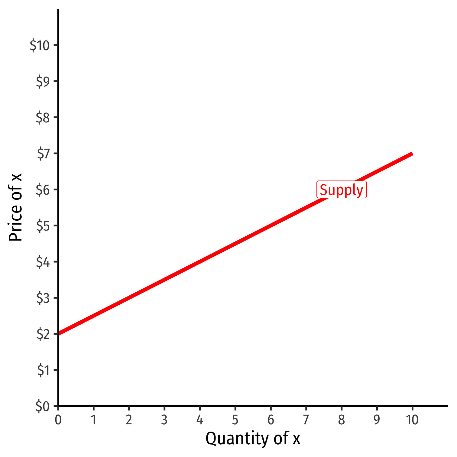
Inverse Supply Function
- Supply demand function relates price to quantity
- Find by taking demand function and solving for p
Example: p=2+0.5q
Graphable (price on vertical axis)!
Slope: 0.5
Vertical intercept called the "Choke price": price where qS=0 ($2), just low enough to discourage any sales

Inverse Supply Function
- Inverse supply function relates price to quantity
- Find by taking suuply function and solving for p
Example: p=2+0.5q
Read two ways:
Horizontally: at any given price, how many units firm wants to sell
Vertically: at any given quantity, the minimum willingness to accept (WTA) for that quantity

Price Elasticity of Supply
- Price elasticity of supply measures how much (in %) quantity supplied changes in response to a (1%) change in price
ϵqS,p=%ΔqS%Δp

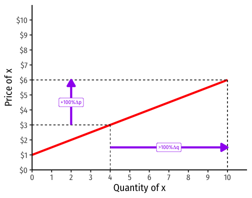
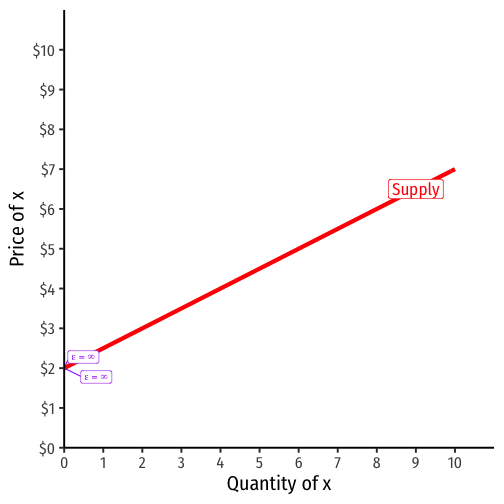
Visualizing Price Elasticity of Supply
An identical 100% price increase on an:
"Inelastic" Supply Curve
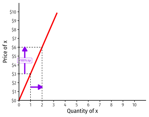
"Elastic" Supply Curve
Price Elasticity of Supply Formula
ϵq,p=1slope×pq
First term is the inverse of the slope of the inverse supply curve (that we graph)!
To find the elasticity at any point, we need 3 things:
- The price
- The associated quantity supplied
- The slope of the (inverse) supply curve
Price Elasticity of Supply Changes Along the Supply Curve
ϵq,p=1slope×pq
Elasticity ≠ slope (but they are related)!
Elasticity changes along the supply curve
Often gets less elastic as ↑ price (↑ quantity)
- Harder to supply more
Determinants of Price Elasticity of Supply I
What determines how responsive your selling behavior is to a price change?
Increasing/Decreasing/Constant Cost industry ⟹ less/more/perfectly elastic supply
- Mining for natural resources vs. automated manufacturing
Smaller (larger) share of market for inputs ⟹ more (less) elastic
- Will your suppliers raise the price much if you buy more?
- How much competition is there in your input markets?
Determinants of Price Elasticity of Supply II
What determines how responsive your selling behavior is to a price change?
- More (less) time to adjust to price changes ⟹ more (less) elastic