Recall: The Firm's Two Problems
- First Stage: the firm's profit maximization problem:
Choose: < output >
In order to maximize: < profits >
- Second Stage: the firm's cost minimization problem:
Choose: < inputs >
In order to minimize: < cost >
Subject to: < producing the optimal output >
- Minimizing costs \(\iff\) maximizing profits

A Competitive Market
- We assume (for now) the firm is in a competitive industry:
Firms' products are perfect substitutes
Firms are "price-takers", no one firm can affect the market price
Market entry and exit are free1

1 Remember this feature. It turns out to be the most important feature that distinguishes different types of industries!
Profit
Recall that profit is is: $$\pi=\underbrace{pq}_{revenues}-\underbrace{(wl+rk)}_{costs}$$
We'll first take a closer look at costs, then at revenues
Next class we'll put them together to find \(q^*\) that maximizes \(\pi\) (the first stage problem)

Costs in Economics are Opportunity Costs
- Costs in economics are different from common conception of "cost"
- Accounting cost: monetary cost
- Economic cost: value of next best use of resources given up (opportunity cost)


Costs in Economics are Opportunity Costs
Costs in economics are different from common conception of "cost"
- Accounting cost: monetary cost
- Economic cost: value of next best use of resources given up
This leads to the difference between
- Accounting profit: revenues minus accounting costs
- Economic profit: revenues minues accounting & opportunity costs
The Accounting vs. Economic Point of View I
- Helpful to consider two points of view:
- "Accounting point of view": are you taking in more cash than you are spending?
- "Economic point of view: is your product you making the best social use of your resources (i.e. are there higher-valued uses of your resources you are keeping them away from)?
The Accounting vs. Economic Point of View II
Social implications: are consumers best off with you using scarce resources (with alternative uses!) to produce your current product?
Remember: this is an economics course, not a business course!
- What might be good/bad for one business might have bad/good consequences for society!
Opportunity Cost is Hard for People

Opportunity Costs vs. Sunk Costs
Opportunity cost is a forward-looking concept
Choices made in the past with non-recoverable costs are called sunk costs
Sunk costs should not enter into future decisions
Many people have difficulty letting go of unchangeable past decisions: sunk cost fallacy

Sunk Costs: Examples

Sunk Costs: Examples

Sunks Costs: Examples

The Sunk Cost Fallacy

Common Sunk Costs in Business
Licensing fees, long-term lease contracts
Specific capital (with no alternative use): uniforms, menus, signs
Research & Development spending
Advertising spending
Fixed vs. Sunk costs
What is the difference between fixed and sunk costs?
Sunk costs are a type of fixed cost that are not avoidable or recoverable
Many fixed costs can be avoided or changed in the long run
Common fixed, but not sunk, costs:
- rent for office space
- durable equipment
- operating permits (that are renewed)
When deciding to stay in business, fixed costs matter, sunk costs do not!
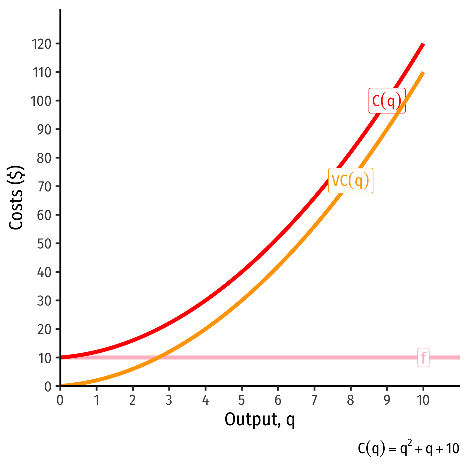
Cost Functions: Example, Visualized
| \(q\) | \(f\) | \(VC(q)\) | \(C(q)\) |
|---|---|---|---|
| \(0\) | \(10\) | \(0\) | \(10\) |
| \(1\) | \(10\) | \(2\) | \(12\) |
| \(2\) | \(10\) | \(6\) | \(16\) |
| \(3\) | \(10\) | \(12\) | \(22\) |
| \(4\) | \(10\) | \(20\) | \(30\) |
| \(5\) | \(10\) | \(30\) | \(40\) |
| \(6\) | \(10\) | \(42\) | \(52\) |
| \(7\) | \(10\) | \(56\) | \(66\) |
| \(8\) | \(10\) | \(72\) | \(82\) |
| \(9\) | \(10\) | \(90\) | \(100\) |
| \(10\) | \(10\) | \(110\) | \(120\) |
The Importance of Marginal Cost

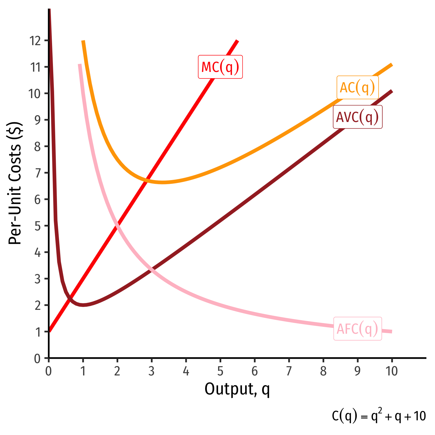
Average and Marginal Costs: Visualized
| \(q\) | \(C(q)\) | \(MC(q)\) | \(AFC(q)\) | \(AVC(q)\) | \(AC(q)\) |
|---|---|---|---|---|---|
| \(0\) | \(10\) | \(-\) | \(-\) | \(-\) | \(-\) |
| \(1\) | \(12\) | \(2\) | \(10.00\) | \(2\) | \(12.00\) |
| \(2\) | \(16\) | \(4\) | \(5.00\) | \(3\) | \(8.00\) |
| \(3\) | \(22\) | \(6\) | \(3.33\) | \(4\) | \(7.30\) |
| \(4\) | \(30\) | \(8\) | \(2.50\) | \(5\) | \(7.50\) |
| \(5\) | \(40\) | \(10\) | \(2.00\) | \(6\) | \(8.00\) |
| \(6\) | \(52\) | \(12\) | \(1.67\) | \(7\) | \(8.70\) |
| \(7\) | \(66\) | \(14\) | \(1.43\) | \(8\) | \(9.40\) |
| \(8\) | \(82\) | \(16\) | \(1.25\) | \(9\) | \(10.25\) |
| \(9\) | \(100\) | \(18\) | \(1.11\) | \(10\) | \(11.10\) |
| \(10\) | \(120\) | \(20\) | \(1.00\) | \(11\) | \(12.00\) |
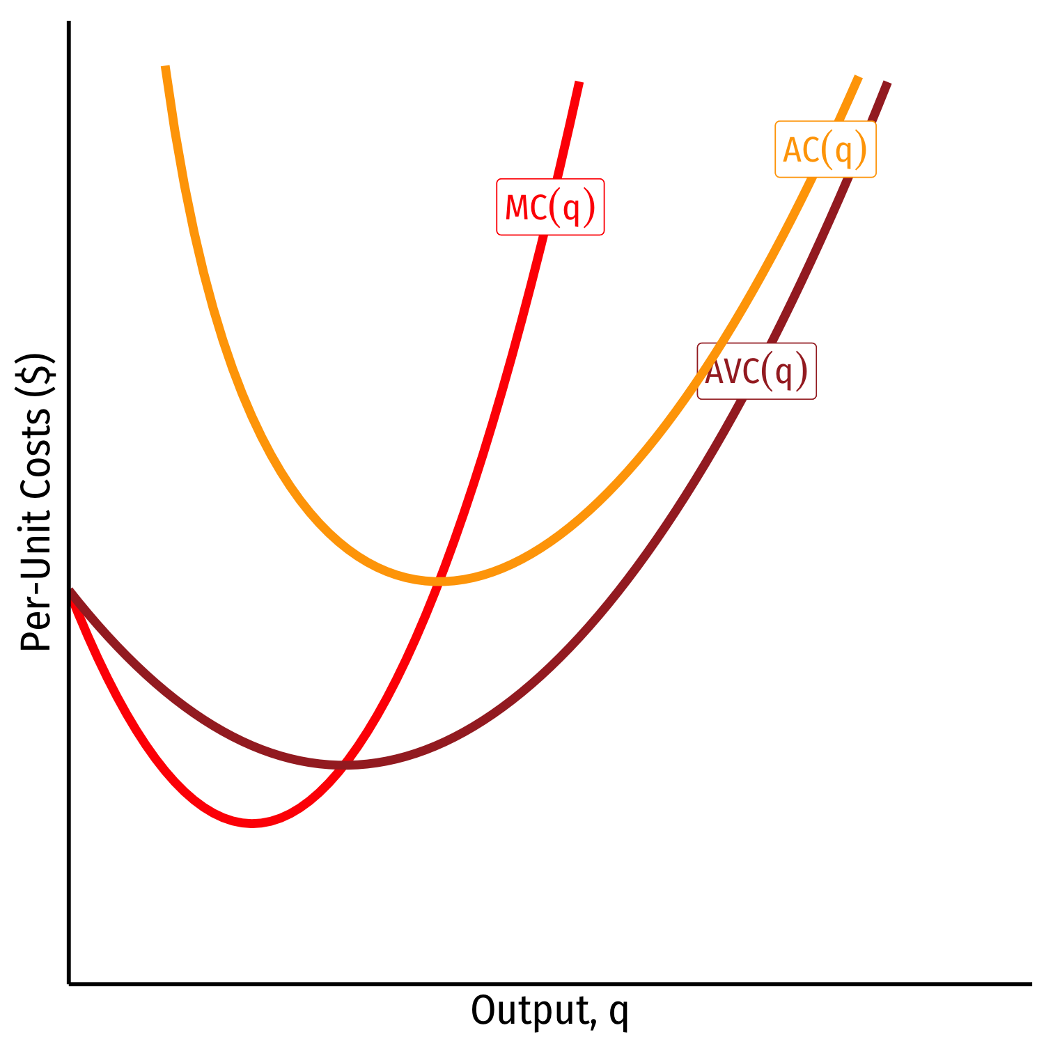
Relationship Between Marginal and Average
There is a general mathematical relationship between a marginal and an average value:
Whenever marginal \(>\) average, average is increasing

Relationship Between Marginal and Average
There is a general mathematical relationship between a marginal and an average value:
Whenever marginal \(>\) average, average is increasing
Whenever marginal \(<\) average, average is decreasing
Relationship Between Marginal and Average
There is a general mathematical relationship between a marginal and an average value:
Whenever marginal \(>\) average, average is increasing
Whenever marginal \(<\) average, average is decreasing
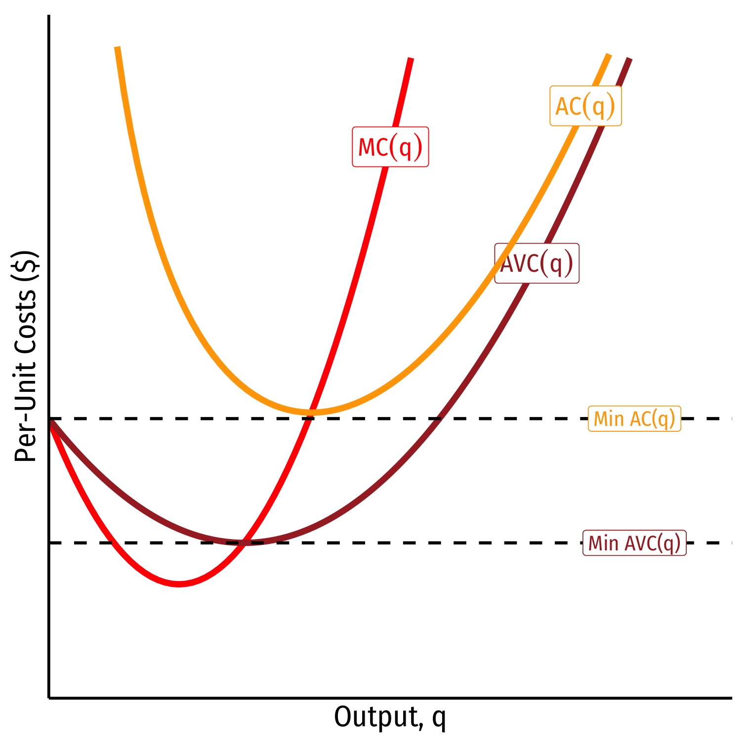
When marginal \(=\) average, average is maximized/minimized
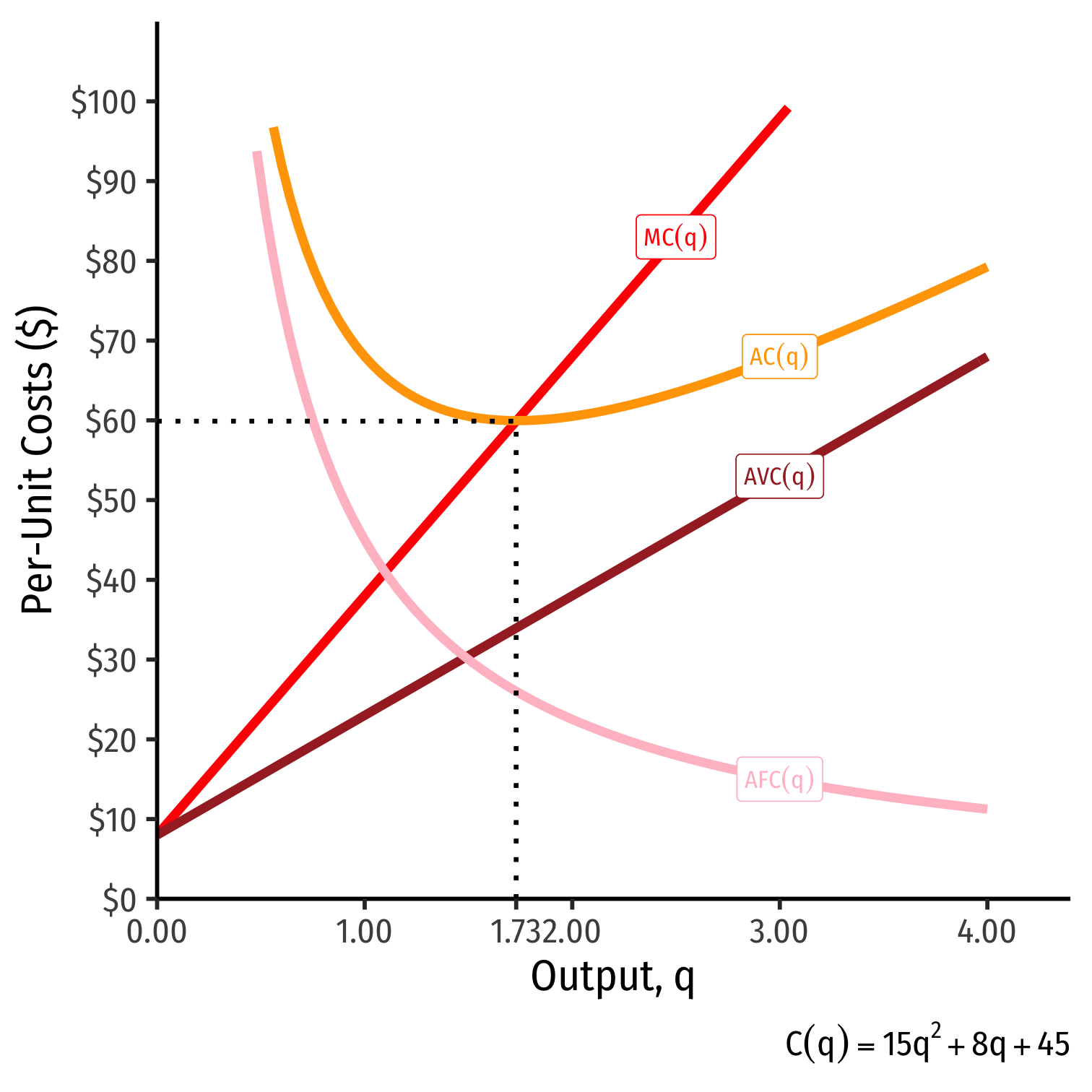
- When \(MC=AC\), \(AC\) is at a minimum
When \(MC=AVC\), \(AVC\) is at a minimum
Economic importance (later):
- Break-even price and shut-down price
Costs: Example: Visualized
Costs in the Long Run
In the long run, firm can change all factors of production, and vary the scale of production
Long run average cost, LRAC(q): cost per unit of output when the firm can change both \(l\) and \(k\) to make more \(q\)
Long run marginal cost, LRMC(q): change in long run total cost as the firm produce an additional unit of \(q\) (by changing both \(l\) and/or \(k\))
Don't worry much about these, they are nearly identical to short run cost curves
One important idea...

Average Cost in the Long Run
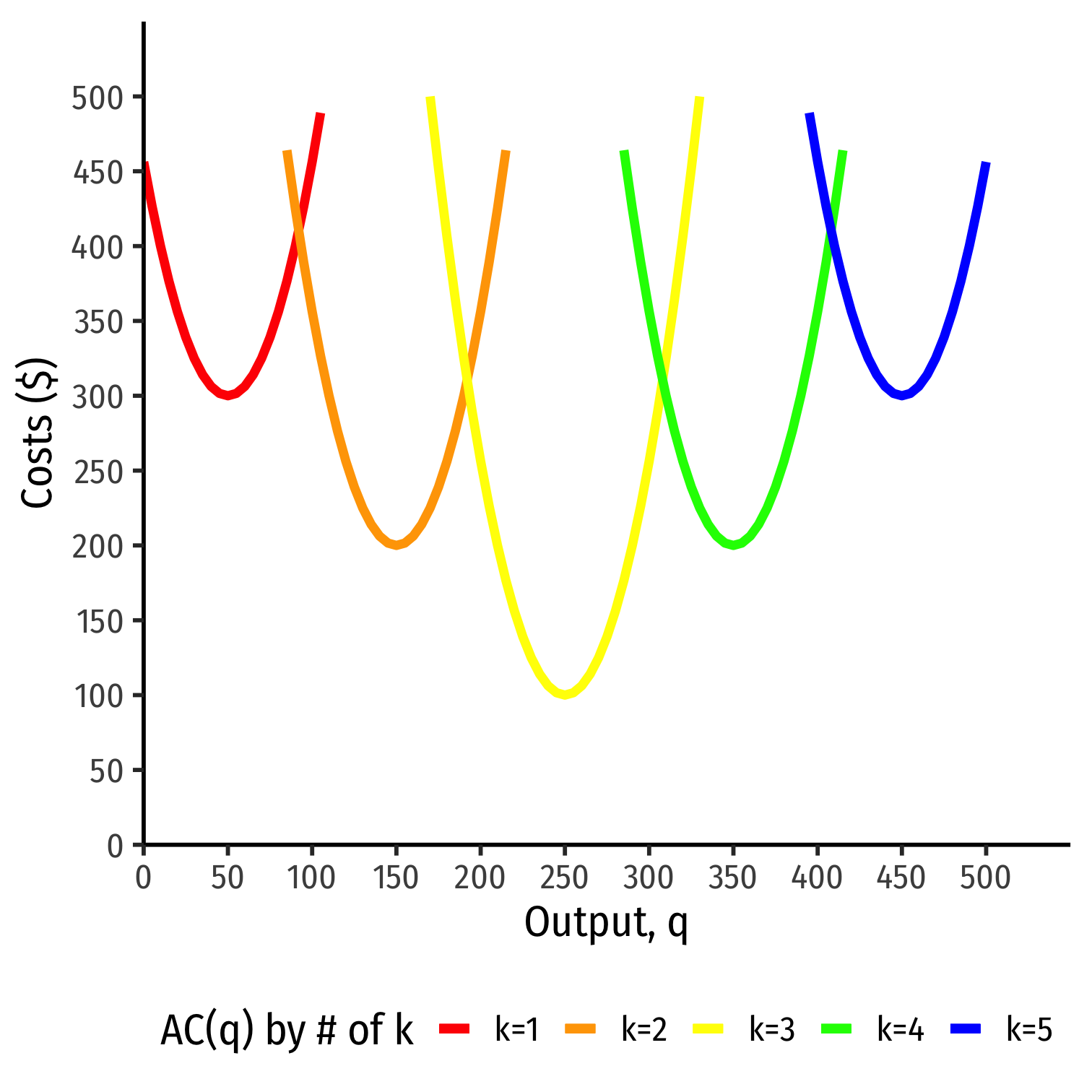
In the long run, firm can choose \(k\) (factories, locations, etc)
Separate short run average cost (SRAC) curves for each amount of \(k\) potentially chosen
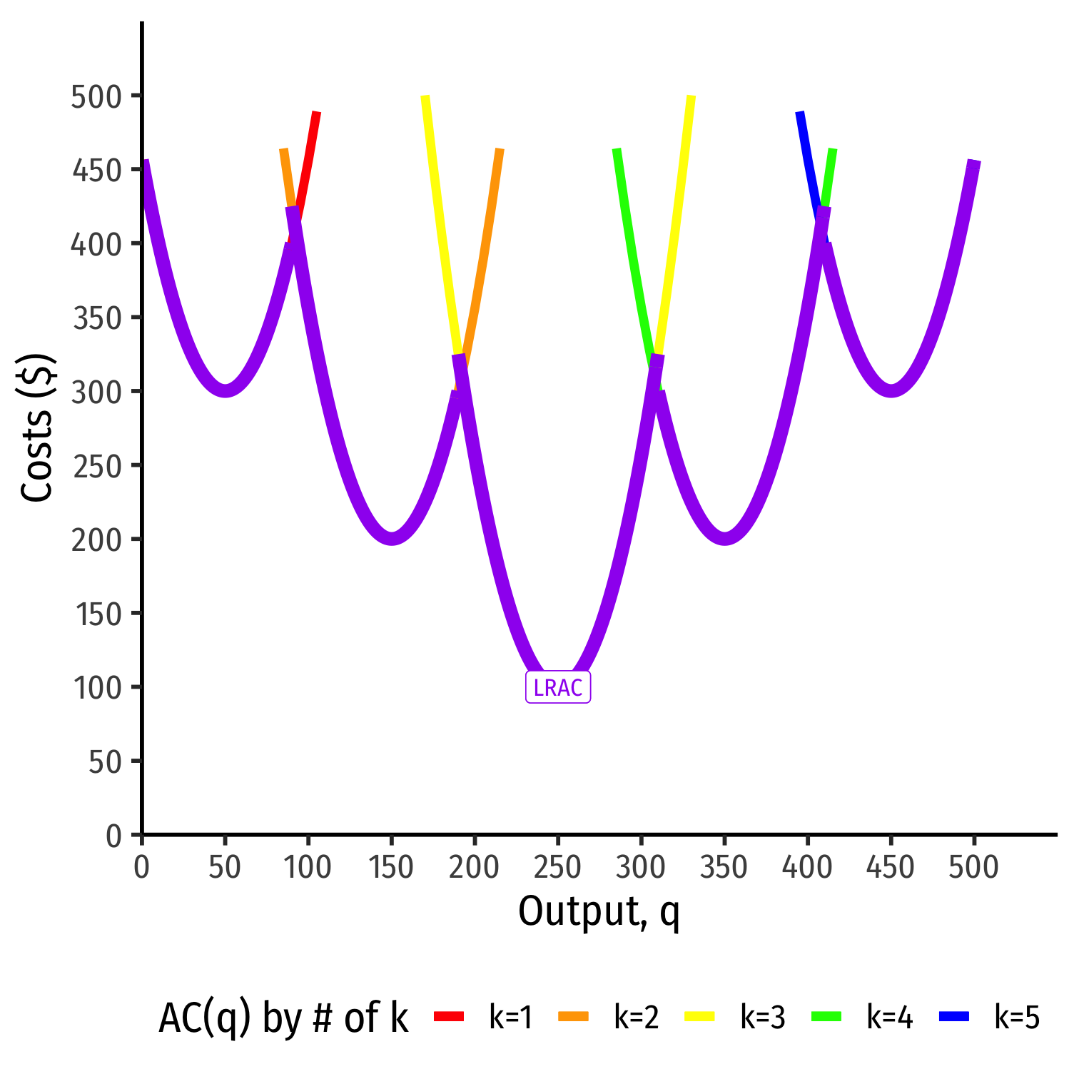
Long run average cost (LRAC) curve "envelopes" the lowest (optimal) parts of all the SRAC curves!
"Subject to producing the optimal amount of output, choose l and k to minimize cost"
Average Cost in the Long Run
In the long run, firm can choose \(k\) (factories, locations, etc)
Separate short run average cost (SRAC) curves for each amount of \(k\) potentially chosen
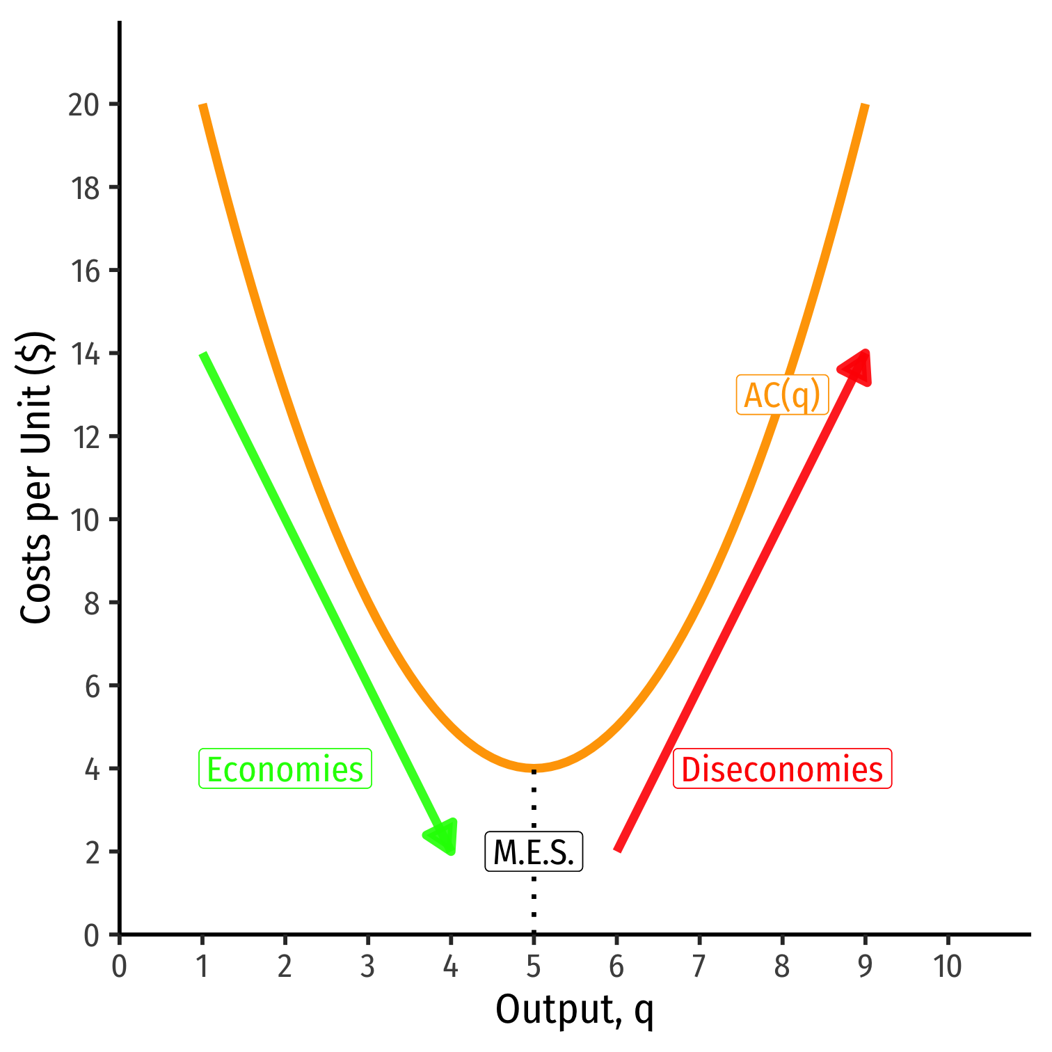
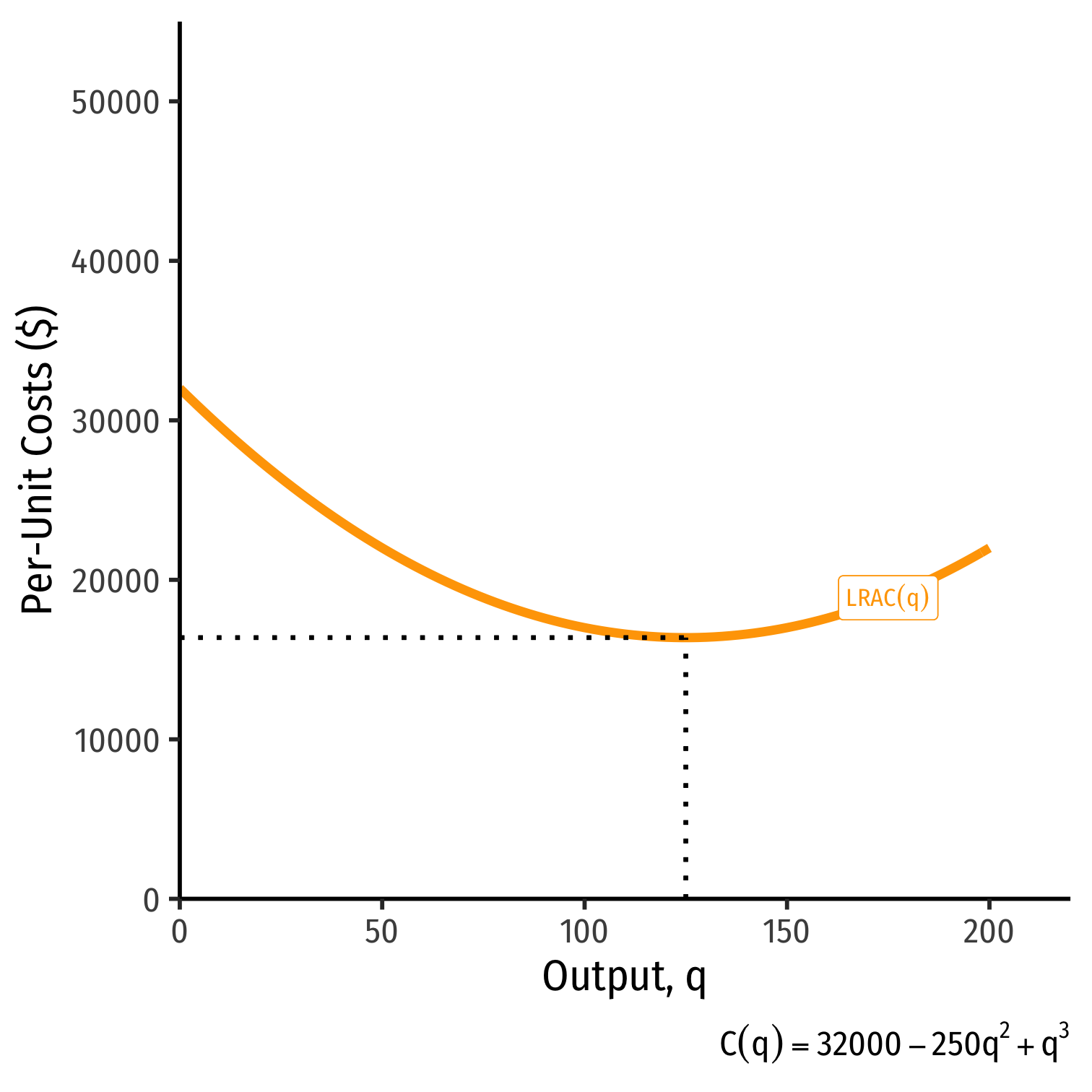
Long Run Costs & Scale Economies II
Minimum Efficient Scale: \(q\) with the lowest \(AC(q)\)
Economies of Scale: \(\uparrow q\), \(\downarrow AC(q)\)
Diseconomies of Scale: \(\uparrow q\), \(\uparrow AC(q)\)
Long Run Costs and Scale Economies: Example, Visualized
Revenues for Firms in Competitive Industries I

Revenues for Firms in Competitive Industries I
Revenues for Firms in Competitive Industries I
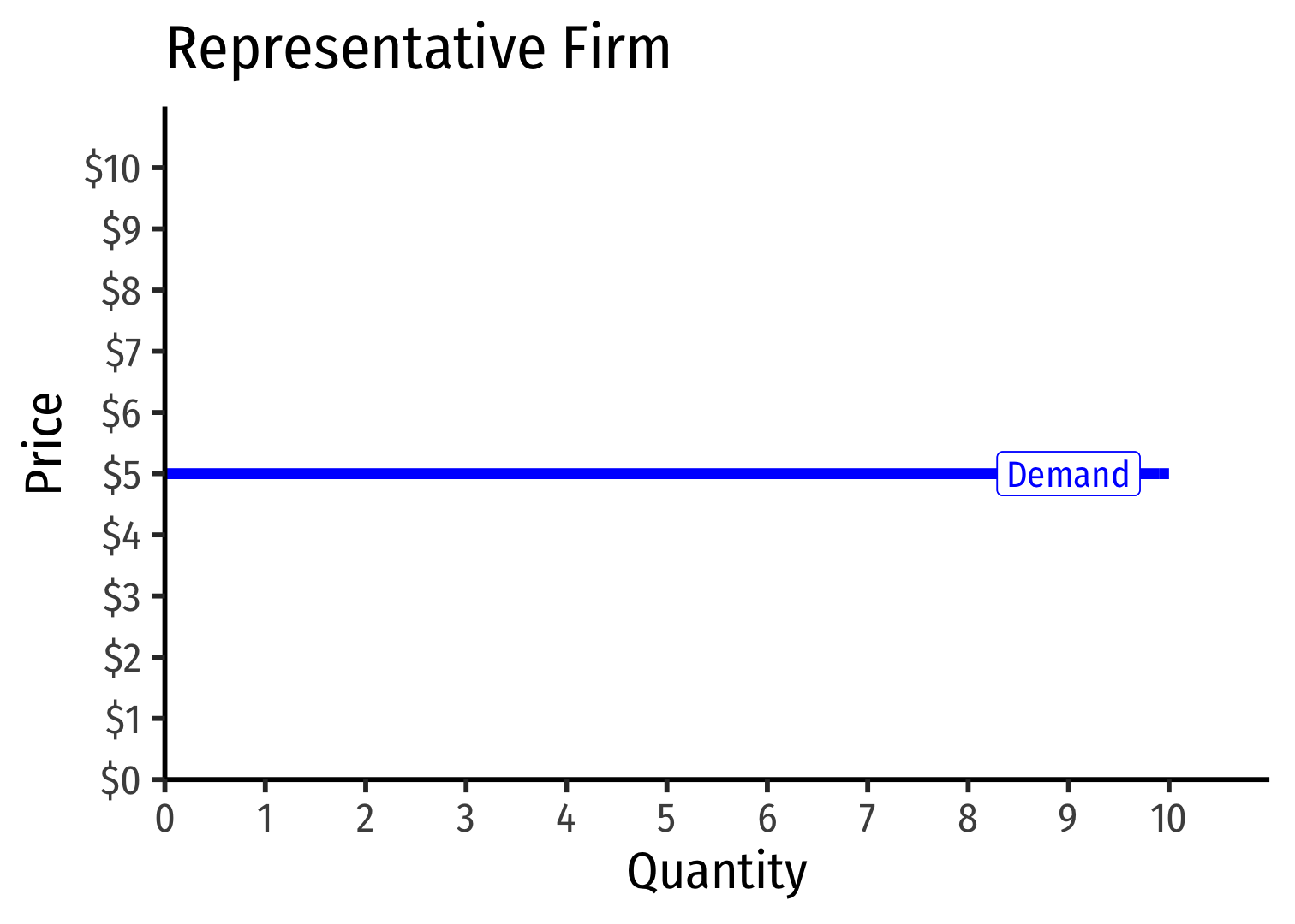
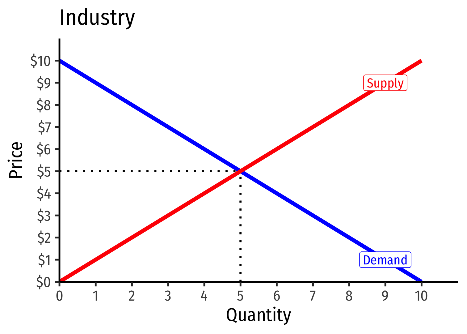
- Demand for a firm's product is perfectly elastic at the market price
Revenues for Firms in Competitive Industries I
Demand for a firm's product is perfectly elastic at the market price
Where did the supply curve come from? You'll see
Revenues for Firms in Competitive Industries II
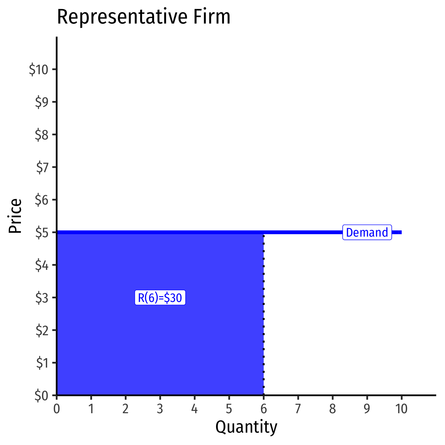
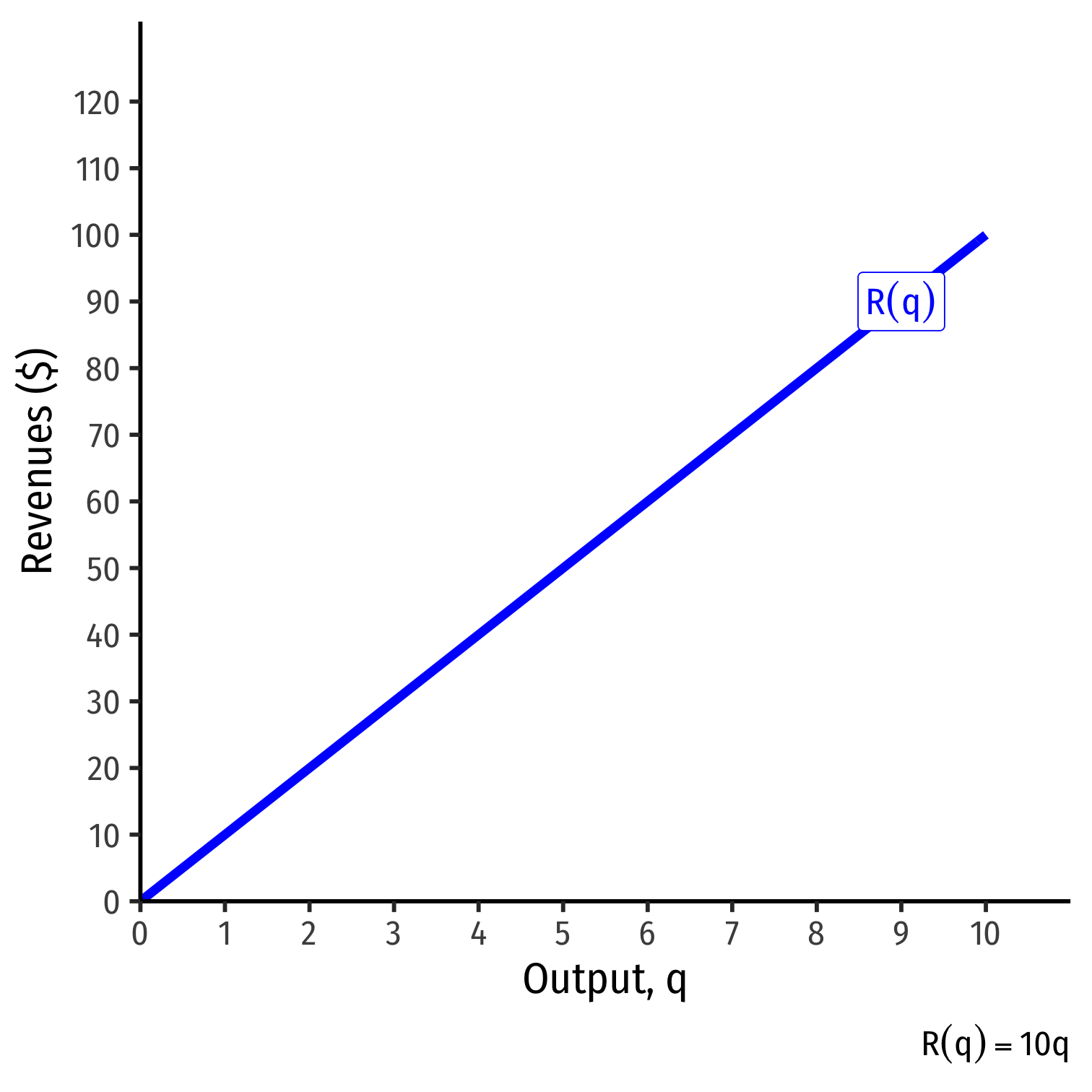
- Total Revenue \(R(q)=pq\)
Total Revenue, Example: Visualized
| \(q\) | \(R(q)\) |
|---|---|
| \(0\) | \(0\) |
| \(1\) | \(10\) |
| \(2\) | \(20\) |
| \(3\) | \(30\) |
| \(4\) | \(40\) |
| \(5\) | \(50\) |
| \(6\) | \(60\) |
| \(7\) | \(70\) |
| \(8\) | \(80\) |
| \(9\) | \(90\) |
| \(10\) | \(100\) |
Average and Marginal Revenue, Example: Visualized
| \(q\) | \(R(q)\) | \(AR(q)\) | \(MR(q)\) |
|---|---|---|---|
| \(0\) | \(0\) | \(-\) | \(-\) |
| \(1\) | \(10\) | \(10\) | \(10\) |
| \(2\) | \(20\) | \(10\) | \(10\) |
| \(3\) | \(30\) | \(10\) | \(10\) |
| \(4\) | \(40\) | \(10\) | \(10\) |
| \(5\) | \(50\) | \(10\) | \(10\) |
| \(6\) | \(60\) | \(10\) | \(10\) |
| \(7\) | \(70\) | \(10\) | \(10\) |
| \(8\) | \(80\) | \(10\) | \(10\) |
| \(9\) | \(90\) | \(10\) | \(10\) |
| \(10\) | \(100\) | \(10\) | \(10\) |
