A Demand Function (Again)
- A consumer's quantity demanded (of good x), qDx is a function of their demand for good x, which depends on current market prices and their income
qDx=D(m,px,py)
- We now want to examine how quantity demanded for x changes as each of these parameters change:
- Income effects (ΔqDxΔm): how qDx changes with changes in income
- Cross-price effects (ΔqDxΔpy): how qDx changes with changes in prices of other goods (e.g. y)
- (Own) Price effects (ΔqDxΔpx): how qDx changes with changes in price (of x)

The (Own) Price Effect
- Price effect: change in optimal consumption of a good associated with a change in its price, holding income and other prices constant
ΔqDxΔpx<0
The law of demand: as the price of a good rises, people will tend to buy less of that good (and vice versa)
- i.e. the price effect is negative!

(Real) Income Effect
Suppose there is only 1 good to consume, x. You have a $100 income, and the price of x is $10. You consume 10 units of x
Suppose the price of x falls to $5. Your now consume 20 units of x.
This is the real income effect: a change in the price of x changes your real income or purchasing power, the amount of goods you can buy
Note your actual (nominal) income of $100 never changed!

(Real) Income Effect: Size
The size of the income effect depends on how large a portion of your budget you spend on the good
Large-budget items:
- e.g. Housing/apartment rent, car prices
- Price increase makes you much poorer
- Price decrease makes you much wealthier
Small-budget items:
- e.g. pencils, toothpicks, candy
- Price changes don't have much of an effect on your wealth or change your behavior much


Substitution Effect
Suppose there are 1000s of goods, none of them are a major fraction of your budget
Suppose the price of one good, x increases
The real income effect for x is tiny (and negative)
But you would consume less of x relative to other goods because x is now relatively more expensive
That's the substitution effect: consumption changes because of a change in relative prices

Substitution Effect: Size
- The size of the substitution effect depends on how substitutable two goods are
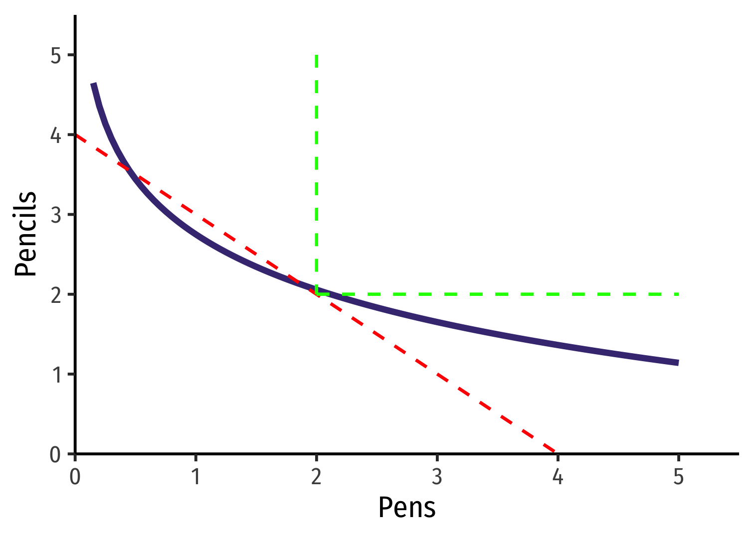
- Straighter → more substitutable
Substitution Effect: Size
- The size of the substitution effect depends on how substitutable two goods are
- Straighter → more substitutable
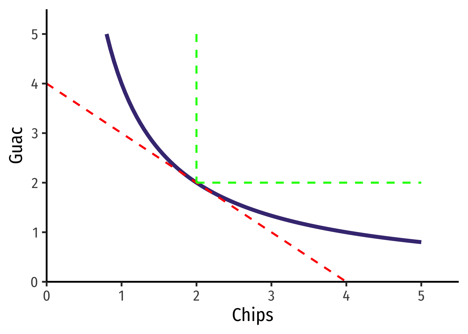
- Curved → more complementary
Real Income and Substitution Effects, Graphically I
- Original optimal consumption (A)
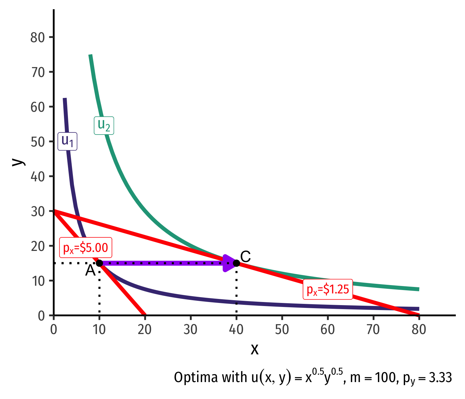
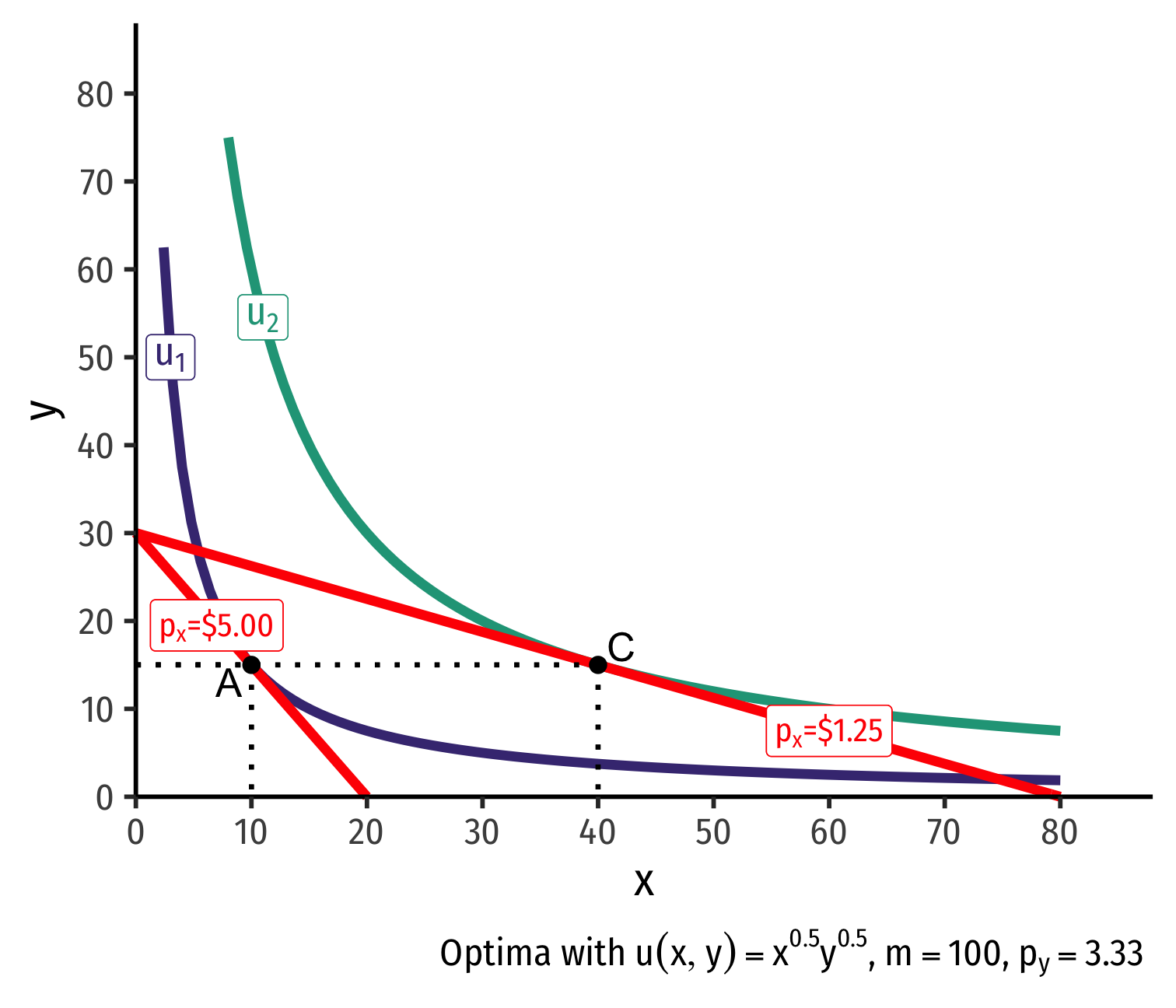
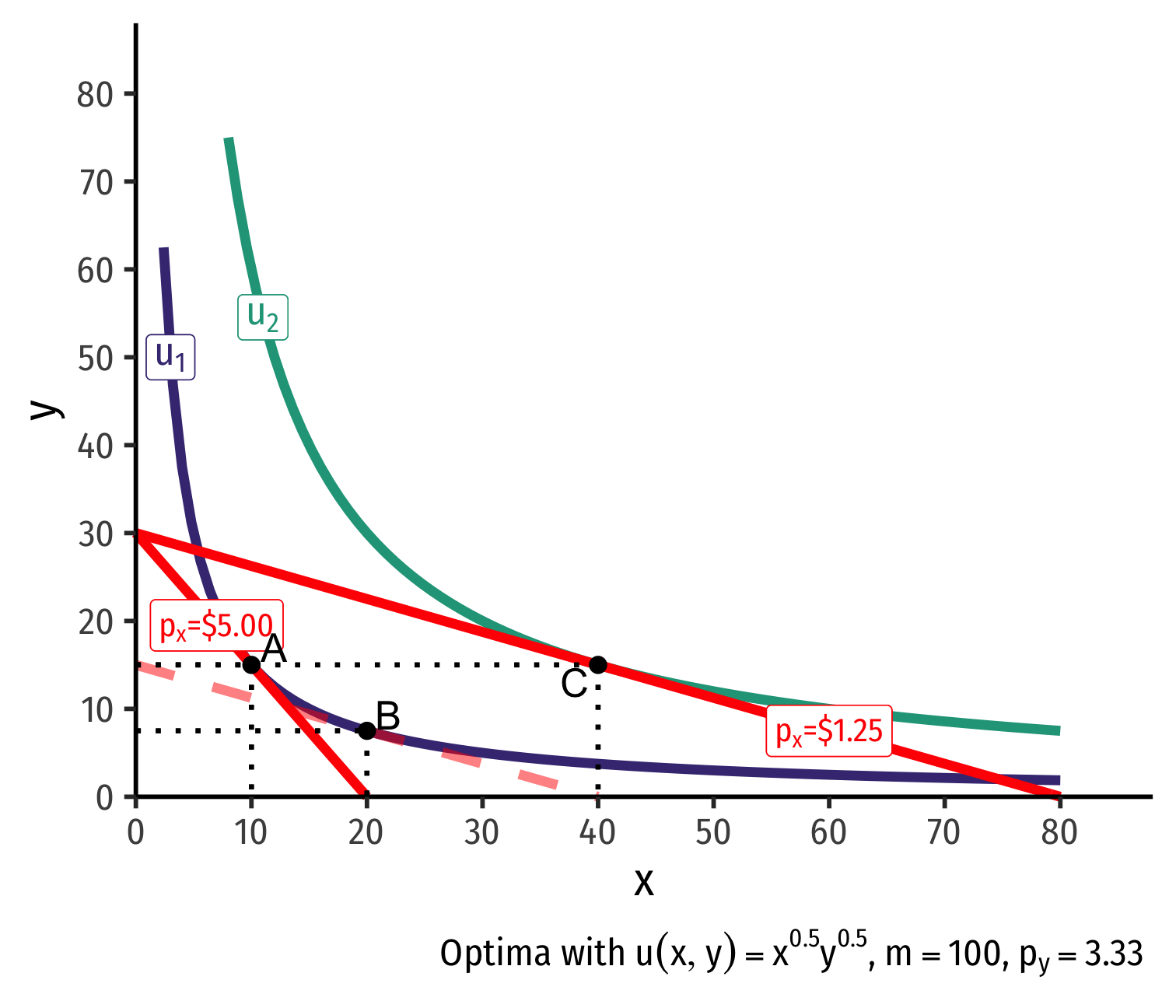
Real Income and Substitution Effects, Graphically I
Original optimal consumption (A)
(Total) price effect: A→C
Let's decompose this into the two effects
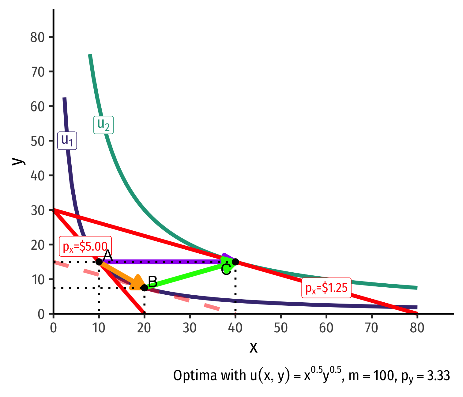
Real Income and Substitution Effects, Graphically II
- Substitution effect: what would have been chosen at the new price ratio to remain indifferent as before
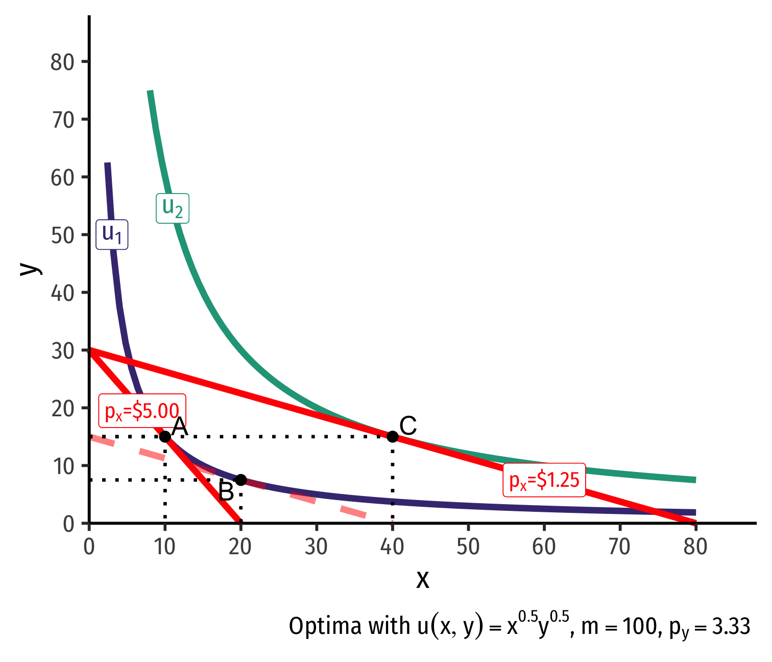
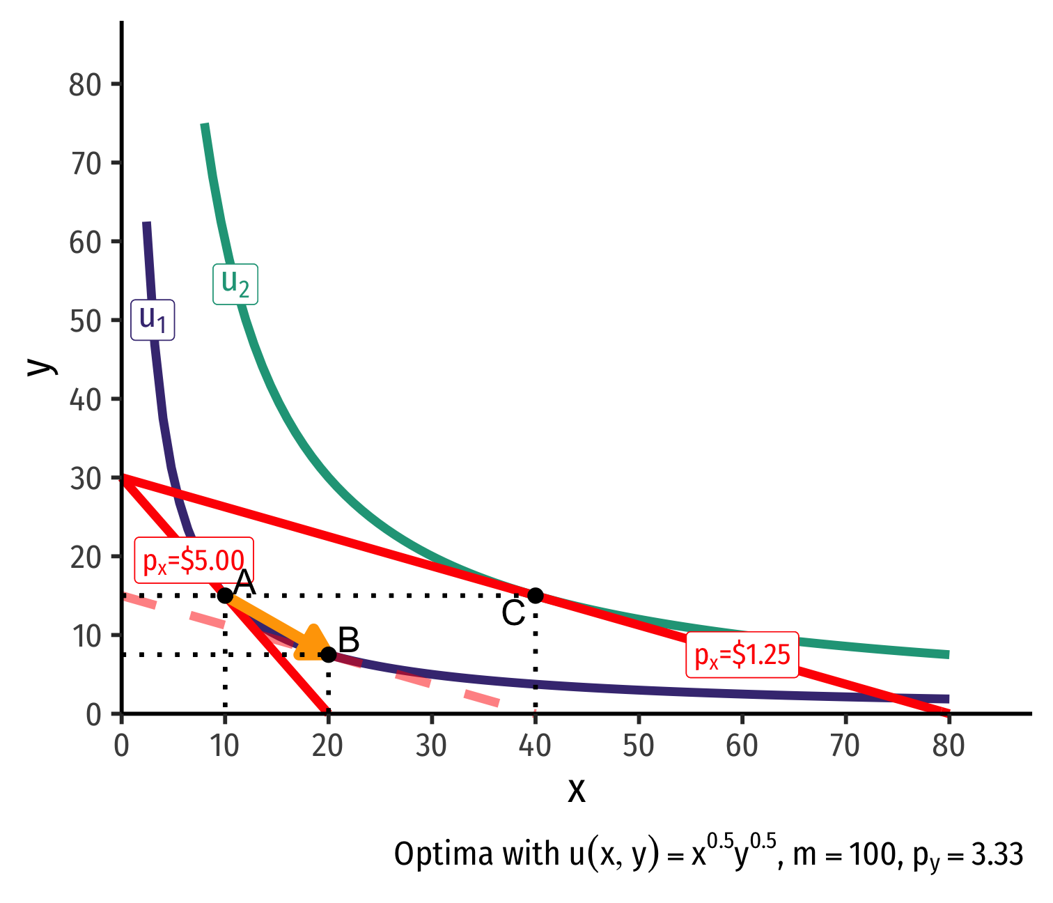
Real Income and Substitution Effects, Graphically II
Substitution effect: what would have been chosen at the new price ratio to remain indifferent as before
Graphically: shift new budget constraint inwards until tangent with old indifference curve
A→B on same I.C. (↑ cheaper x and ↓ y)
- Note it must be a different point on the original curve!
Real Income and Substitution Effects, Graphically III
- (Real) income effect: change in quantities consumed due to the change in purchasing power after the change in price

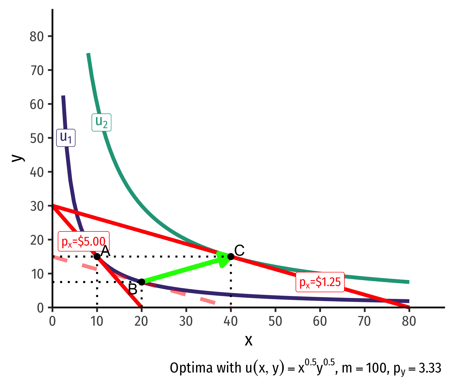
Real Income and Substitution Effects, Graphically III
(Real) income effect: change in quantities consumed due to the change in purchasing power after the change in price
B→C to new budget constraint (can buy more of x and/or y)
Real Income and Substitution Effects, Graphically III
(Real) income effect: change in quantities consumed due to the change in purchasing power after the change in price
B→C to new budget constraint (can buy more of x and/or y)
Real Income and Substitution Effects, Graphically IV
- Original optimal consumption (A)

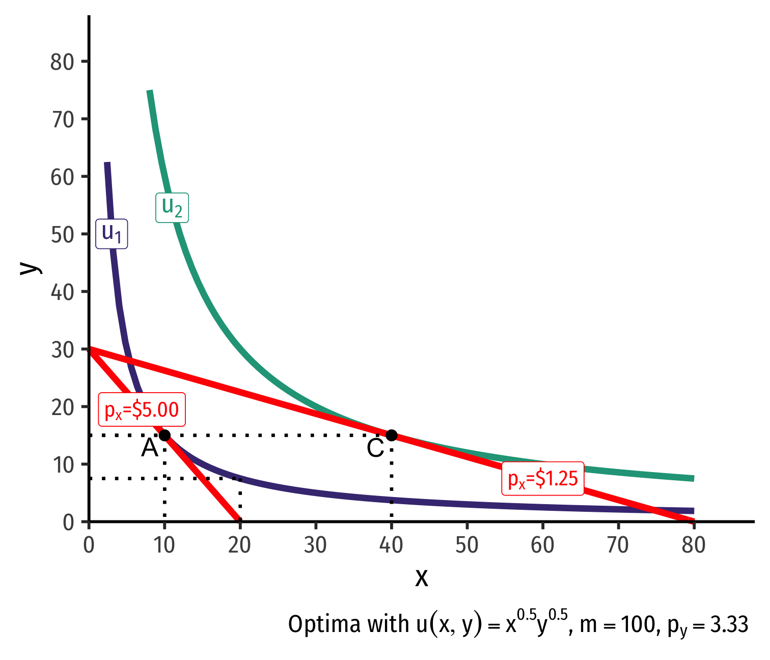
Real Income and Substitution Effects, Graphically IV
Original optimal consumption (A)
Price of x falls, new optimal consumption at (C)
Real Income and Substitution Effects, Graphically IV
Original optimal consumption (A)
Price of x falls, new optimal consumption at (C)
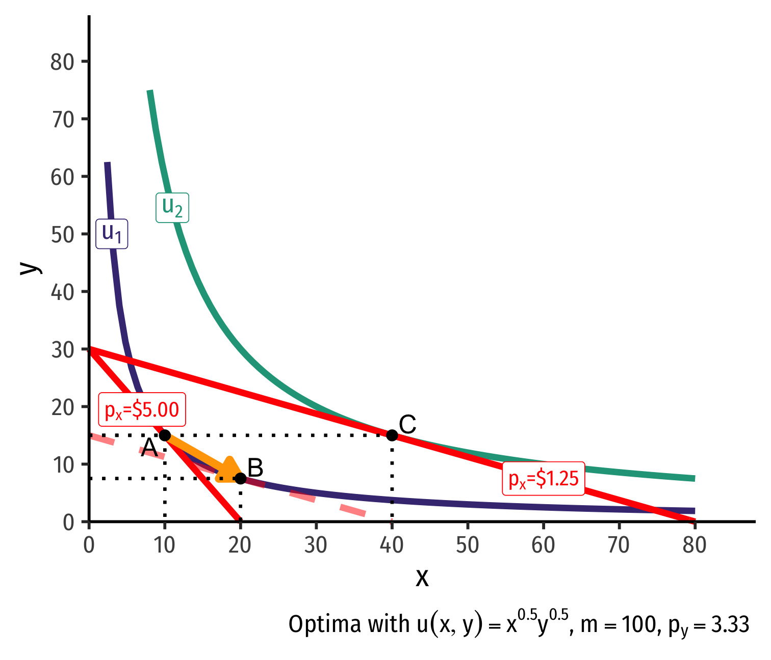
Substitution effect: A→B on same I.C. (↑ cheaper x and ↓ y)
Real Income and Substitution Effects, Graphically IV
Original optimal consumption (A)
Price of x falls, new optimal consumption at (C)
Substitution effect: A→B on same I.C. (↑ cheaper x and ↓ y)
(Real) income effect: B→C to new budget constraint (can buy more of x and/or y)
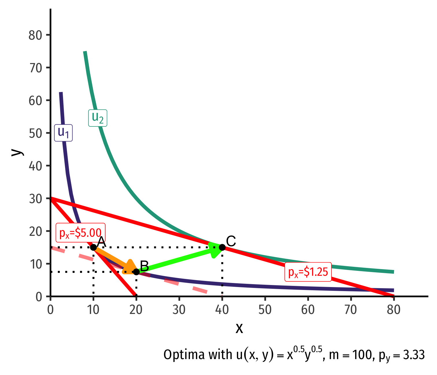
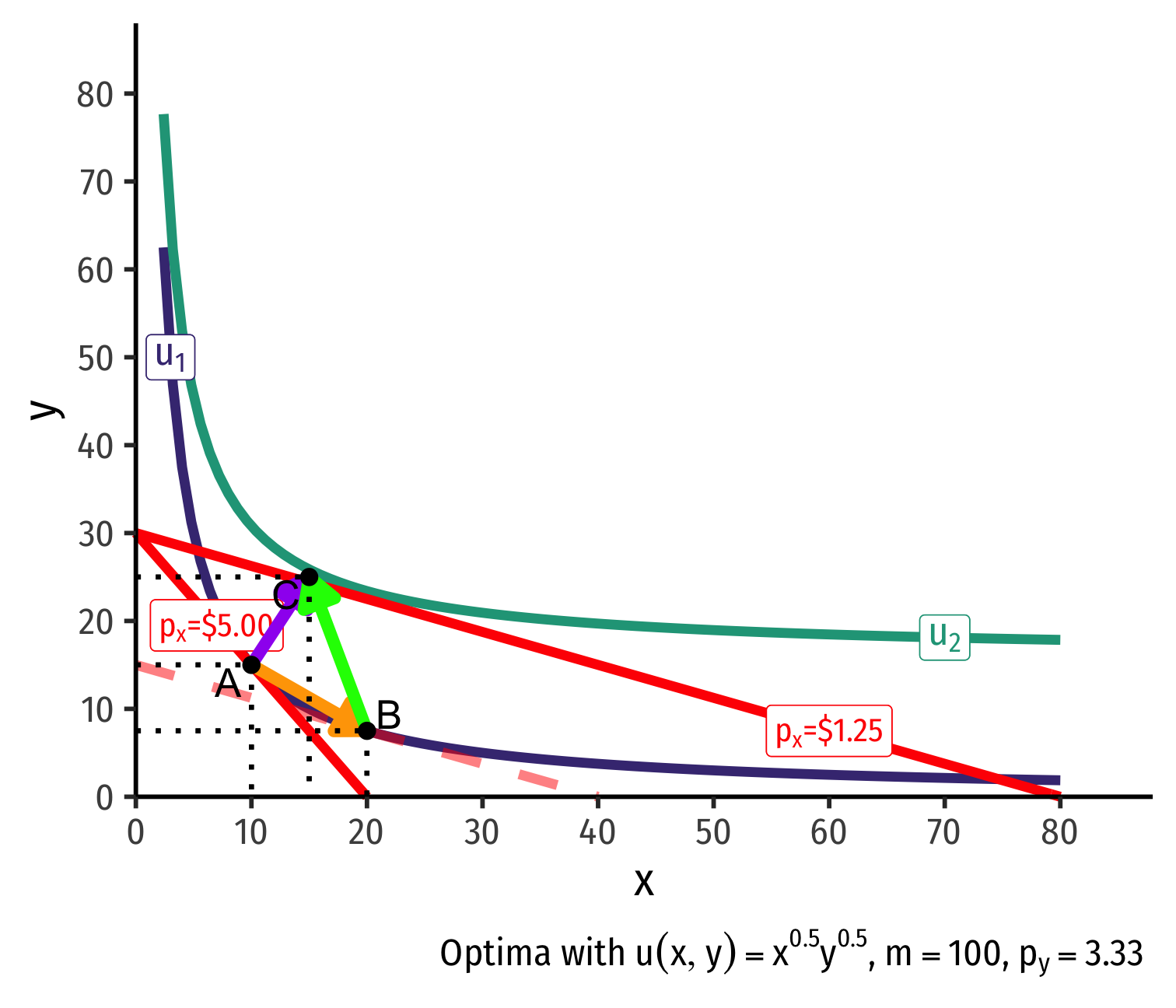
Real Income and Substitution Effects, Graphically IV
Original optimal consumption (A)
Price of x falls, new optimal consumption at (C)
Substitution effect: A→B on same I.C. (↑ cheaper x and ↓ y)
(Real) income effect: B→C to new budget constraint (can buy more of x and/or y)
(Total) price effect: A→C
Real Income and Substitution Effects: Inferior Good
- What about for an inferior good (like Ramen)?
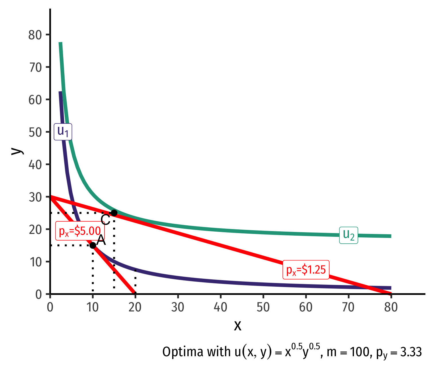
Real Income and Substitution Effects: Inferior Good
What about for an inferior good (like Ramen)?
Substitution effect: A→B on same I.C. (↑ cheaper x and ↓ y)
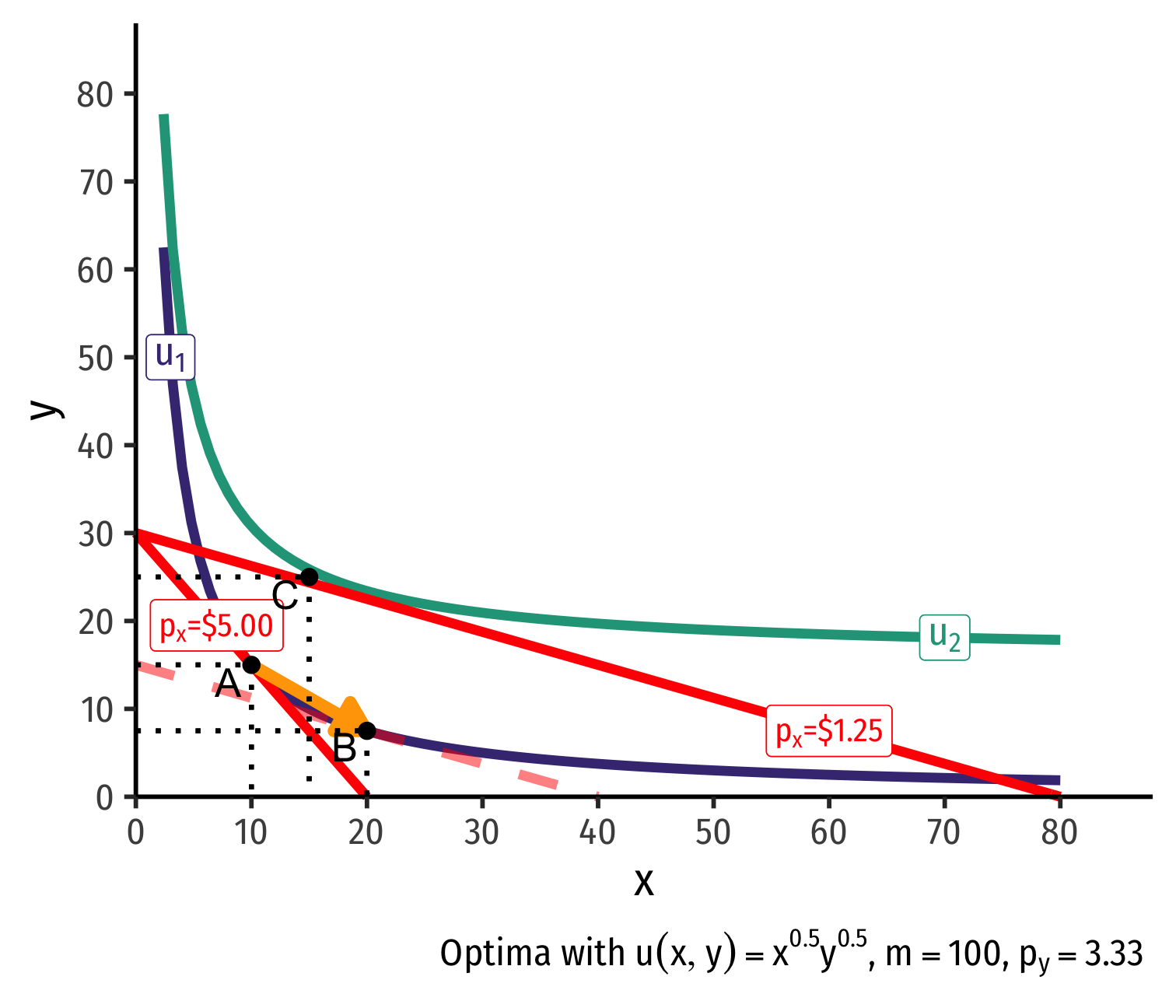
Real Income and Substitution Effects: Inferior Good
What about for an inferior good (like Ramen)?
Substitution effect: A→B on same I.C. (↑ cheaper x and ↓ y)
(Real) income effect: B→C to new budget constraint (can buy more of x and/or y)

Real Income and Substitution Effects: Inferior Good
What about for an inferior good (like Ramen)?
Substitution effect: A→B on same I.C. (↑ cheaper x and ↓ y)
(Real) income effect: B→C to new budget constraint (can buy more of x and/or y)
(Total) price effect: A→C

Real Income and Substitution Effects: Inferior Good
What about for an inferior good (like Ramen)?
Substitution effect: A→B on same I.C. (↑ cheaper x and ↓ y)
(Real) income effect: B→C to new budget constraint (can buy more of x and/or y)
(Total) price effect: A→C
Price effect is still an ↑x from a ↓px!
- Person would just prefer to spend more new purchasing power on other goods (y)!
The law of demand holds, even for inferior goods!
- Because subst. effect dominates real income effect
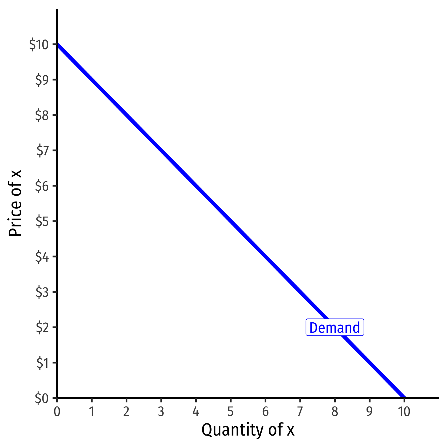
Demand Curve
Demand curve graphically represents the demand schedule
Also measures a person's maximum willingness to pay (WTP) for a given quantity
Law of Demand (price effect) ⟹ Demand curves always slope downwards

Demand Function
- Demand function relates quantity to price
Example: q=10−p
- Not graphable (wrong axes)!

Inverse Demand Function
- Inverse demand function relates price to quantity
- Find by taking demand function and solving for p
Example: p=10−q
Graphable (price on vertical axis)!
Slope: −1
Vertical intercept called the "Choke price": price where qD=0 ($10), just high enough to discourage any purchases

Inverse Demand Function
- Inverse demand function relates price to quantity
- Find by taking demand function and solving for p
Example: p=10−q
Read two ways:
Horizontally: at any given price, how many units person wants to buy
Vertically: at any given quantity, the maximum willingness to pay (WTP) for that quantity
- This way will be very useful later
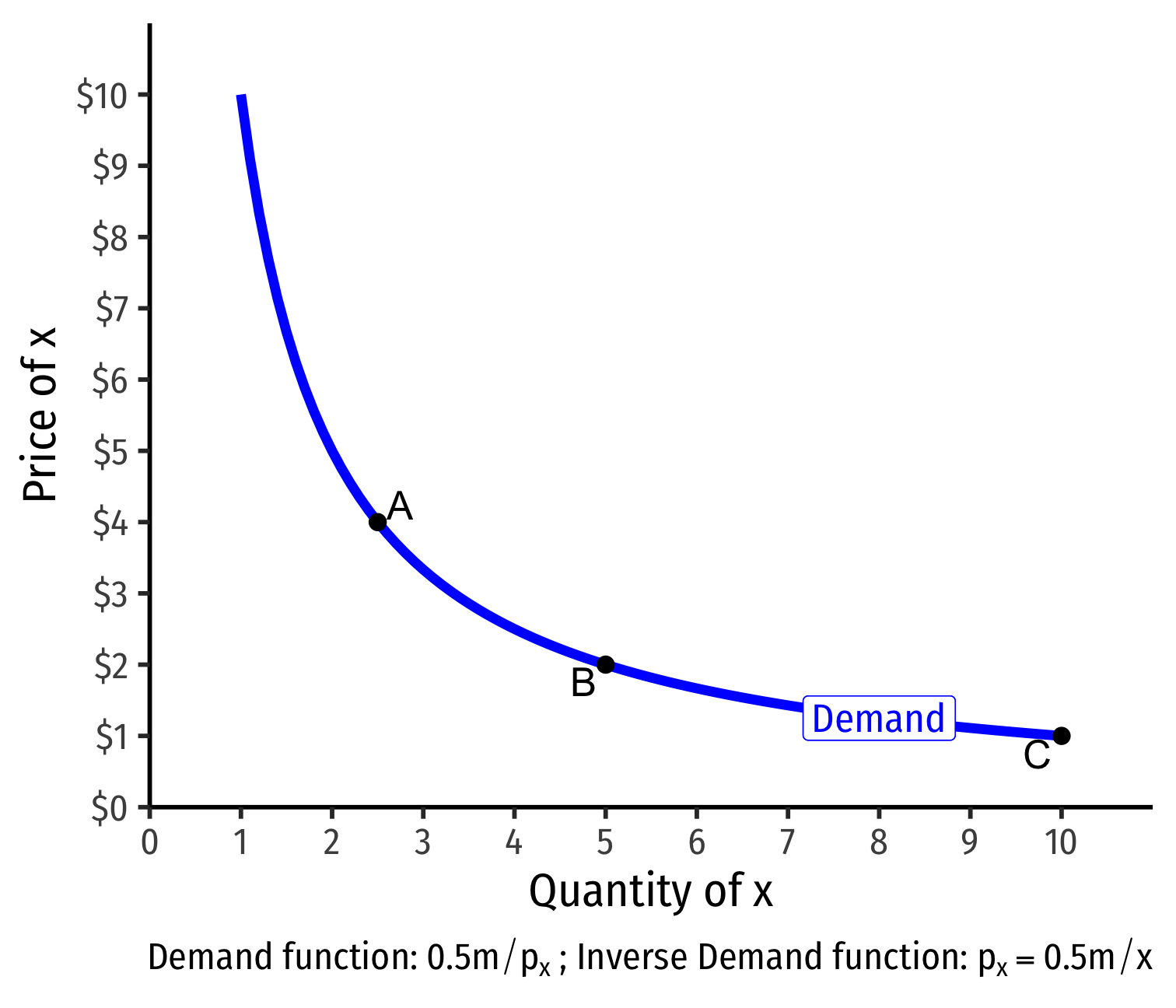
Deriving a Demand Curve Graphically
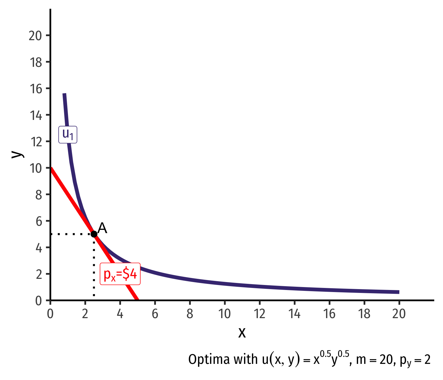
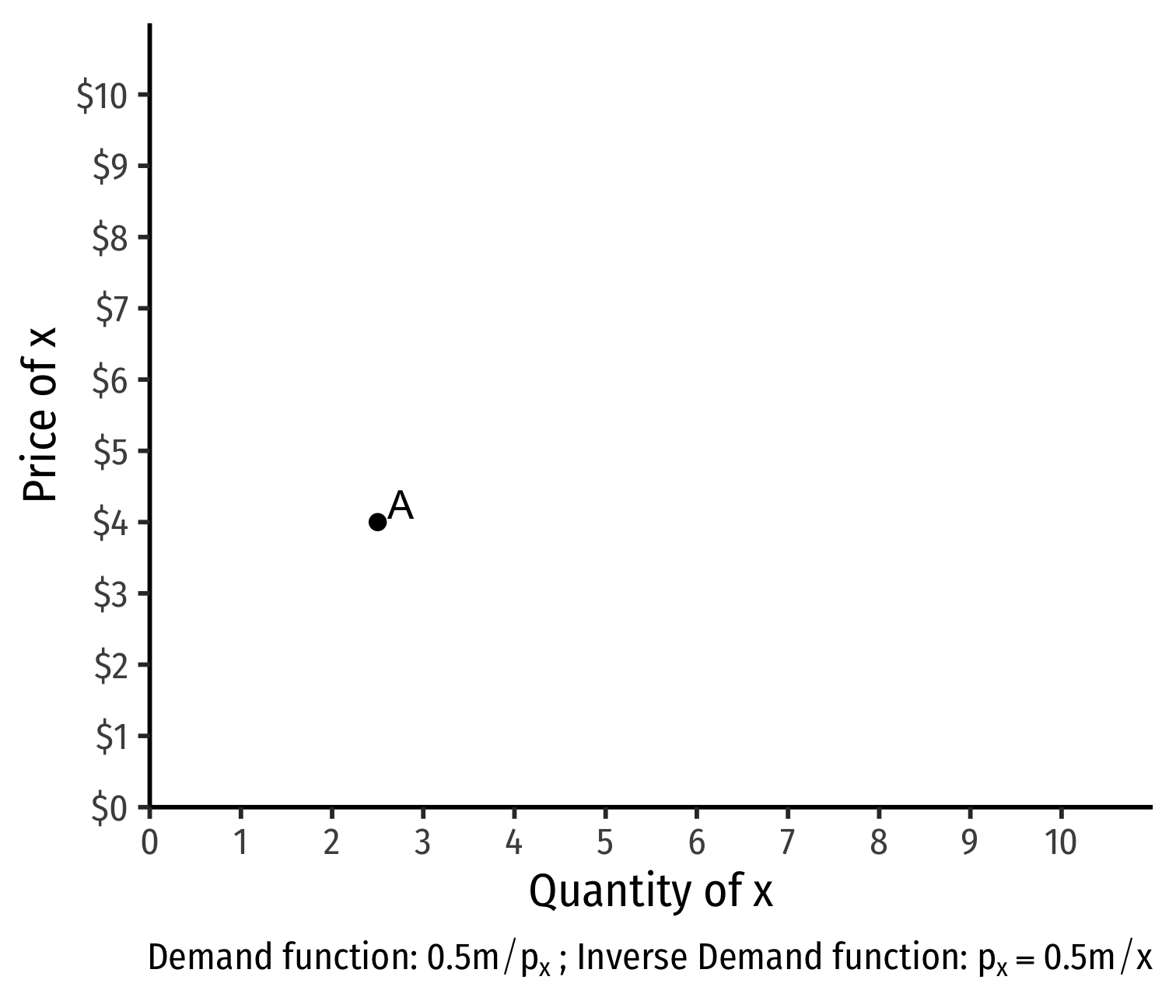
- Demand curve for x relates consumer's optimal consumption of x ("quantity") as price of x changes
- At px=4, consumer buys 2 x
Deriving a Demand Curve Graphically
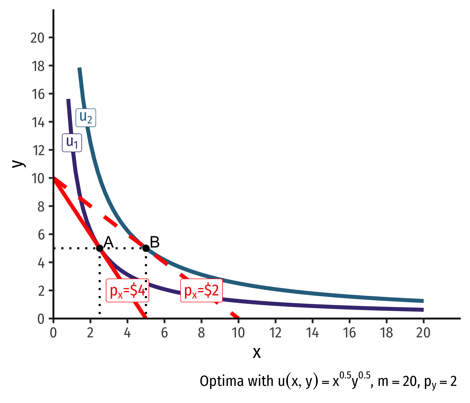
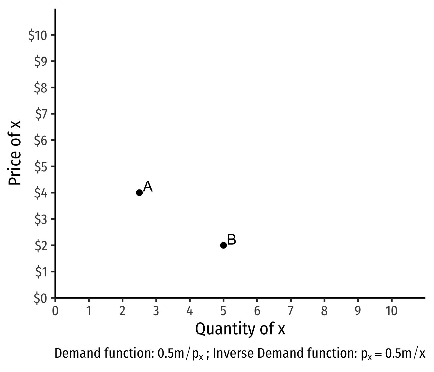
- Demand curve for x relates consumer's optimal consumption of x ("quantity") as price of x changes
- At px=4, consumer buys 2 x; at px=2, consumer buys 5 x
Deriving a Demand Curve Graphically
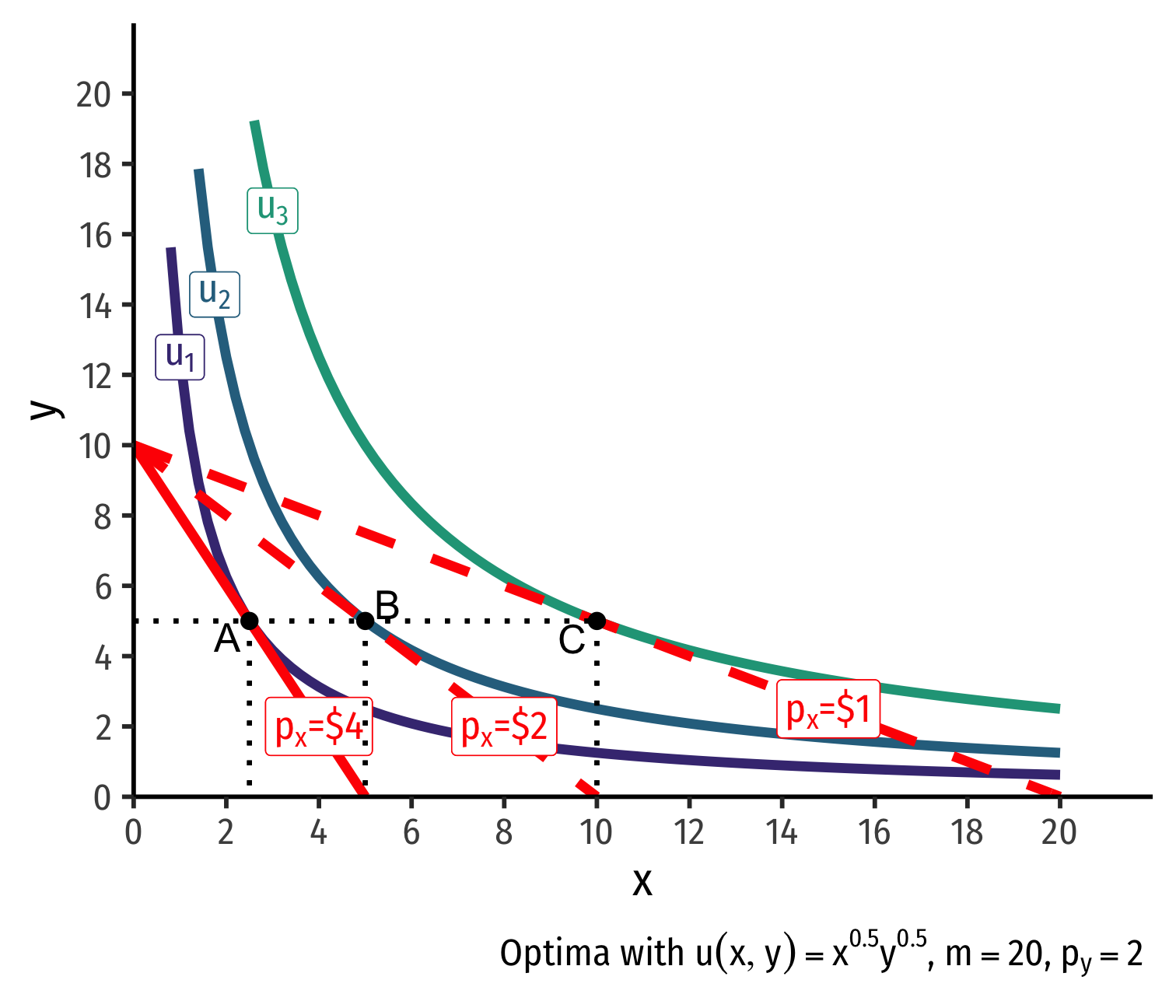
- Demand curve for x relates consumer's optimal consumption of x ("quantity") as price of x changes
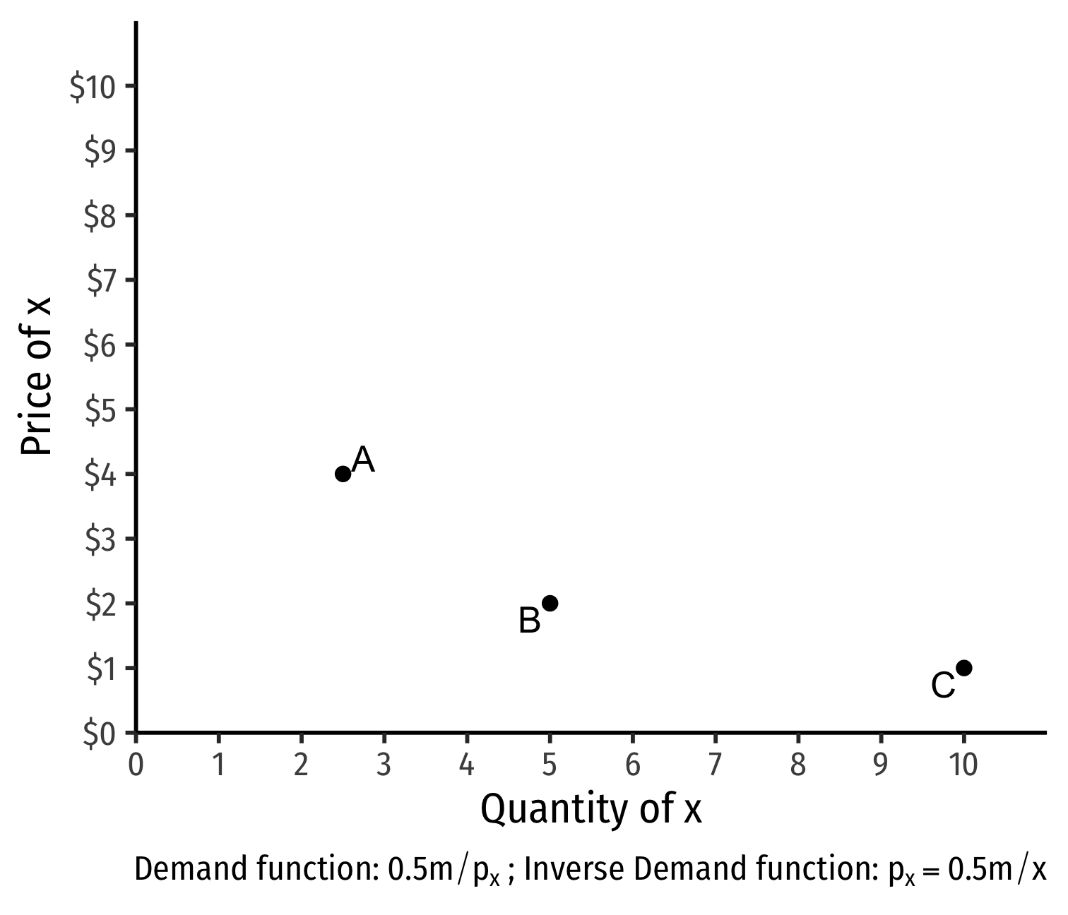
- At px=4, consumer buys 2 x; at px=2, consumer buys 5 x; at px=1, consumer buys 10 x
Deriving a Demand Curve Graphically

- Demand curve for x relates consumer's optimal consumption of x ("quantity") as price of x changes
- At px=4, consumer buys 2 x; at px=2, consumer buys 5 x; at px=1, consumer buys 10 x
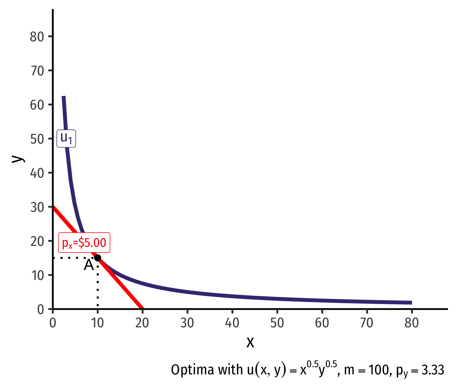
Deriving a Demand Function III
Example: u(x,y)=x0.5y0.5, demand function is
qx=0.5mpx
Always spend 50% (a) of income on x
With an income of m=10 Demand: qx=5pxInv. demand: px=5qx
With an income of m=50 Demand: qx=25pxInv. demand: px=25qx
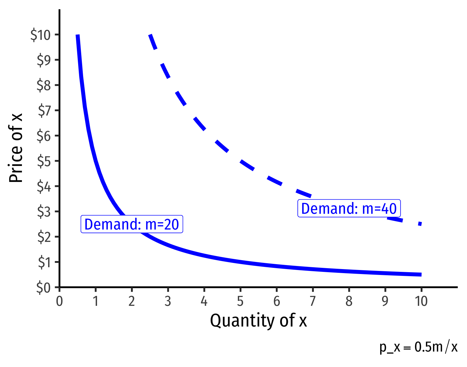
Shifts in Demand I
- Note a simple (inverse) demand function only relates (own) price and quantity
Example: q=10−p or p=10−q
What about all the other "determinants of demand" like income and other prices?
They are captured in the vertical intercept (choke price)!

Shifts in Demand I
- Note a simple (inverse) demand function only relates (own) price and quantity
Example: q=10−p or p=10−q
What about all the other "determinants of demand" like income and other prices?
They are captured in the vertical intercept (choke price)!

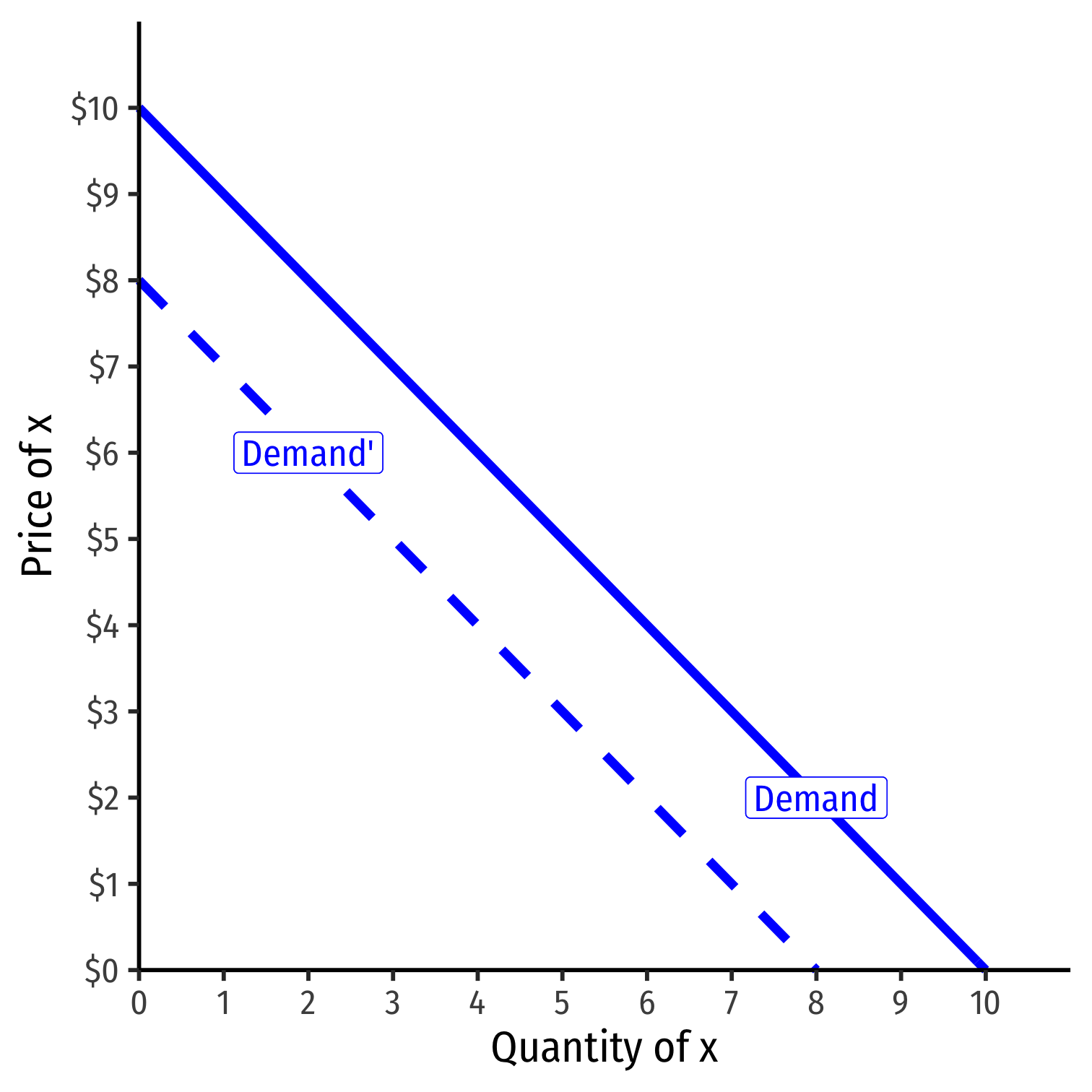
Shifts in Demand II
A change in one of the "determinants of demand" (or "shifters") will shift the demand curve
- Change in income m
- Change in price of other goods py (substitutes or complements)
- Change in preferences or expectations about good x (show up in utility function)
- Change in number of buyers in market
Shows up in (inverse) demand function by a change in the intercept (choke price)!
See my Visualizing Demand Shifters